Extraordinary Popular Miscarriages of Science (part 1)
Posted by Bill Storage in History of Science, Uncategorized on January 18, 2024
By Bill Storage, Jan. 18, 2024
I’ve been collecting examples of bad science. Many came from friends and scientists I’ve talked to. Bad science can cover several aspects of science depending on what one means by science. At least three very different things are called science now:
- An approach or set of rules and methods used to understand and predict nature
- A body of knowledge about nature and natural processes
- An institution, culture or community of people, including academic, government and corporate professionals, who are involved, or are said to be involved, in 1. or 2. above
Many of my examples of bad science fall under the 3rd category and involve, or are dominated by, the academicians, government offices, and corporations. Below are a few of my favorites from the past century or so. I think many people tend to think that bad science happened in medieval times and that the modern western world is immune to that sort of thing. On the contrary, bad science may be on the rise. For the record, I don’t judge a theory bad merely because it was shown to be wrong, even if spectacularly wrong. Geocentricity was a good theory. Phlogiston (17th century theoretical substance believed to escape from matter during combustion), caloric theory (18th century theory of a weightless fluid that flows from hot matter to cold), and the luminiferous ether (17-19th century postulated medium for the propagation of light waves) were all good theories, though we now have robust evidence against them. All had substantial predictive power. All posited unobservable entities to explain phenomena. But predictive success alone cannot justify belief in unobservable entities. Creation science and astrology were always bad science.
To clarify the distinction between bad science and wrong theories, consider Trofim Lysenko. He was nominally a scientist. Some of his theories appear to be right. He wore the uniform, held the office, and published sciencey papers. But he did not behave scientifically (consistent with definition 1 above) when he ignored the boundless evidence and prior art about heredity. Wikipedia dubs him a pseudoscientist, despite his having some successful theories and making testable hypotheses. Pseudoscience, says Wikipedia, makes unfalsifiable claims. Lysenko’s bold claims were falsifiable, and they were falsified. Wikipedia talks as if the demarcation problem – knowing science from pseudoscience – is a closed case. Nah. Rather than tackle that matter of metaphysics and philosophy, I’ll offer that Lysenkoism, like creation science, and astrology, are all sciences but they are bad science. While they all make some testable predictions, they also make a lot of vague ones, their interest in causation is puny, and their research agendas are scant.
Good science entails testable, falsifiable theories and bold predictions. Most philosophers of science, notably excluding Karl Popper, who thought that only withstanding falsification mattered, have held that making succinct, correct prediction makes a theory good, and that successful theories make for good science. Larry Laudan gave, in my view, a fine definition of a successful theory in his 1984 Philosophy of Science: A theory is successful provided it makes substantially more correct predictions, that it leads to efficacious interventions in the natural order, or that it passes a suitable battery of tests.
Concerns over positing unobservables opens a debate on the question of just how observable are electrons, quarks, and the Higgs Field. Not here though. I am more interested in bad science (in the larger senses of science) than I am with wrong theories. Badness often stems not from seeking to explain and predict nature and failing out of refusal to read the evidence fairly, but from cloaking a non-scientific agenda in the trappings of science. I’m interested in what Kuhn, Feyerabend, and Lakatos dealt with – the non-scientific interests of academicians, government offices, and corporations and their impact on what gets studied and how it gets studied, how confirming evidence is sought and processed, how disconfirming evidence is processed, avoided, or dismissed, and whether Popperian falsifiability was ever on the table.
Recap of Kuhn, Feyerabend, and Lakatos
Thomas Kuhn claimed that normal (day-to-day lab-coat) science consisted of showing how nature can be fit into the existing theory. That is, normal science is decidedly unscientific. It is bad science, aimed at protecting the reigning paradigm from disconfirming evidence. On Kuhn’s view, your scientific education teaches you how to see things as your field requires them to be seen. He noted that medieval and renaissance astronomers never saw the supernovae that were seen in China. Europeans “knew” that the heavens were unchanging. Kuhn used the terms dogma and indoctrination to piss off scientists of his day. He thought that during scientific crises (Newton vs. Einstein being the exemplar) scientists clutched at new theories, often irrationally, and then vicious competition ended when scientific methods determined the winner of a new paradigm. Kuhn was, unknown to most of his social-science groupies, a firm believer that the scientific enterprise ultimately worked. Kuhn says normal science is bad science. He thought this was okay because crisis science reverted to good science, and in crisis, the paradigm was overthrown when the scientists got interested in philosophy of science. When Kuhn was all the rage in the early 1960s, radical sociologists of science, all at the time very left leaning, had their doubts that science could stay good under the influence of government and business. Recall worries about the military industrial complex. They thought that interest, whether economic or political, could keep science bad. I think history has sided with those sociologists; though today’s professional sociologists, now overwhelmingly employed by the the US and state governments, are astonishingly silent on the matter. Granting, for sake of argument, that social science is science, its practitioners seem to be living proof that interest can dominate not only research agendas but what counts as evidence, along with the handling of evidence toward what becomes dogma in the paradigm.
Paul Feyerabend, though also no enemy of science, thought Kuhn stopped short of exposing the biggest problems with science. Feyerabend called science, referring to science as an institution, a threat to democracy. He called for “a separation of state and science just as there is a separation between state and religious institutions.” He thought that 1960s institutional science resembled more the church of Galileo’s day than it resembled Galileo. Feyerabend thought theories should be tested against each other, not merely against the world. He called institutional science a threat because it increasingly held complete control over what is deemed scientifically important for society. Historically, he observed, individuals, by voting with their attention and their dollars, have chosen what counts as being socially valuable. Feyerabend leaned rather far left. In my History of Science appointment at UC Berkeley I was often challenged for invoking him against bad-science environmentalism because Feyerabend wouldn’t have supported a right-winger. Such is the state of H of S at Berkeley, now subsumed by Science and Technology Studies, i.e., same social studies bullshit (it all ends in “Studies”), different pile. John Heilbronn rest in peace.
Imre Lakatos had been imprisoned by the Nazis for revisionism. Through that experience he saw Kuhn’s assent of the relevant community as a valid criterion for establishing a new post-crisis paradigm as not much of a virtue. It sounded a bit too much like Nazis and risked becoming “mob psychology.” If the relevant community has excessive organizational or political power, it can put overpowering demands on individual scientists and force them to subordinate their ideas to the community (see String Theory’s attack on Lee Smolin below). Lakatos saw the quality of a science’s research agenda as a strong indicator of quality. Thin research agendas, like those of astrology and creation science, revealed bad science.
Selected Bad Science
Race Science and Eugenics
Eugenics is an all time favorite, not just of mine. It is a poster child for evil-agenda science driven by a fascist. That seems enough knowledge of the matter for the average student of political science. But eugenics did not emerge from fascism and support for it was overwhelming in progressive circles, particularly in American universities and the liberal elite. Alfred Binet of IQ-test fame, H. G. Wells, Margaret Sanger, John Harvey Kellogg, George Bernard Shaw, Theodore Roosevelt, and apparently Oliver Wendell Holmes, based on his decision that compulsory sterilization was within a state’s rights, found eugenics attractive. Financial support for the eugenics movement included the Carnegie Foundation, Rockefeller Institute, and the State Department. Harvard endorsed it, as did Stanford’s first president, David S Jordan. Yale’s famed economist and social reformer Irving Fisher was a supporter. Most aspects of eugenics in the United States ended abruptly when we discovered that Hitler had embraced it and was using it to defend the extermination of Jews. Hitler borrowed from our 1933 Law for the Prevention of Hereditarily Defective Offspring drawn up by Harry Laughlin. Eugenics was a class case of advocates and activists, clueless of any sense of science, broadcasting that the science (the term “race science” exploded onto the scene as if if had always been a thing) had been settled. In an era where many Americans enjoy blaming the living – and some of the living enjoy accepting that blame – for the sins of our fathers, one wonders why these noble academic institutions have not come forth to offer recompense for their eugenics transgressions.
The War on Fat
In 1977 a Senate committee led by George McGovern published “Dietary Goals for the United States,” imploring us to eat less red meat, eggs, and dairy products. The U.S. Department of Agriculture (USDA) then issued its first dietary guidelines, which focused on cutting cholesterol and not only meat fat but fat from any source. The National Institutes of Health recommended that all Americans, including young kids, cut fat consumption. In 1980 the US government broadcast that eating less fat and cholesterol would reduce your risk of heart attack. Evidence then and ever since has not supported this edict. A low-fat diet was alleged to mitigate many metabolic risk factors and to be essential for achieving a healthy body weight. However, over the past 45 years, obesity in the US climbed dramatically while dietary fat levels fell. Europeans with higher fat diets, having the same genetic makeup, are far thinner. The science of low-fat diets and the tenets of related institutions like insurance, healthcare, and school lunches have seemed utterly immune to evidence. Word is finally trickling out. The NIH has not begged pardon.
The DDT Ban
Rachel Carson appeared before the Department of Commerce in 1963, asking for a “Pesticide Commission” to regulate the DDT. Ten years later, Carson’s “Pesticide Commission” became the Environmental Protection Agency, which banned DDT in the US. The rest of the world followed, including Africa, which was bullied by European environmentalists and aid agencies to do so.
By 1960, DDT use had eliminated malaria from eleven countries. Crop production, land values, and personal wealth rose. In eight years of DDT use, Nepal’s malaria rate dropped from over two million to 2,500. Life expectancy rose from 28 to 42 years.
Malaria reemerged when DDT was banned. Since the ban, tens of millions of people have died from malaria. Following Rachel Carson’s Silent Spring narrative, environmentalists claimed that, with DDT, cancer deaths would have negated the malaria survival rates. No evidence supported this. It was fiction invented by Carson. The only type of cancer that increased during DDT use in the US was lung cancer, which correlated cigarette use. But Carson instructed citizens and governments that DDT caused leukemia, liver disease, birth defects, premature births, and other chronic illnesses. If you “know” that DDT altered the structure of eggs, causing bird populations to dwindle, it is Carson’s doing.
Banning DDT didn’t save the birds, because DDT wasn’t the cause of US bird death as Carson reported. While bird populations had plunged prior to DDT’s first use, the bird death at the center of her impassioned plea never happened. We know this from bird count data and many subsequent studies. Carson, in her work at Fish and Wildlife Service and through her participation in Audubon bird counts, certainly knew that during US DDT use, the eagle population doubled, and robin, dove, and catbird counts increased by 500%. Carson lied like hell and we showered her with praise and money. Africans paid with their lives.
In 1969 the Environmental Defense Fund demanded a hearing on DDT. The 8-month investigation concluded DDT was not mutagenic or teratogenic. No cancer, no birth defects. In found no “deleterious effect on freshwater fish, estuarine organisms, wild birds or other wildlife.” Yet William Ruckleshaus, first director of the EPA, who never read the transcript, chose to ban DDT anyway. Joni Mitchell was thrilled. DDT was replaced by more harmful pesticides. NPR, the NY Times, and the Puget Sound Institute still report a “preponderance of evidence” of DDT’s dangers.
When challenged with the claim that DDT never killed kids, the Rachel Carson Landmark Alliance responded in 2017 that indeed it had. A two-year old drank and ounce of 5% DDT in a solution of kerosene and died. Now there’s scientific integrity.
Vilification of Cannabis
I got this one from my dentist; I had never considered it before. White-collar, or rather, work-from-home, California potheads think this problem has been overcome. Far from it. Cannabis use violates federal law. Republicans are too stupid to repeal it, and Democrats are too afraid of looking like hippies. According to Quest Diagnostics, in 2020, 4.4% of workers failed their employers’ drug tests. Blue-collar Americans, particularly those who might be a sub-sub-subcontractor on a government project, are subject to drug tests. Testing positive for weed can cost you your job. So instead of partying on pot, the shop floor consumes immense amounts of alcohol, increasing its risk of accidents at work and in the car, harming its health, and raising its risk of hard drug use. To the admittedly small sense in which the concept of a gateway drug is valid, marijuana is probably not one and alcohol almost certainly is. Racism, big pharma lobbyists, and social-control are typically blamed for keeping cannabis illegal. Governments may also have concluded that tolerating weed at the state level while maintaining federal prohibition is an optimal tax revenue strategy. Cannabis tolerance at state level appears to have reduced opioid use and opioid related ER admissions.
Stoners who scoff at anti-cannabis propaganda like Reefer Madness might be unaware that a strong correlation between psychosis and cannabis use has been known for decades. But inferring causation from that correlation was always either highly insincere (huh huh) or very bad science. Recent analysis of study participants’ genomes showed that those with the strongest genetic profile for schizophrenia were also more likely to use cannabis in large amounts. So unless you follow Lysenko, who thought acquired traits were passed to offspring, pot is unlikely to cause psychosis. When A and B correlate, either A causes B, B causes A, or C causes both, as appears to be the case with schizophrenic potheads.
To be continued.
Settled State Science
Posted by Bill Storage in History of Science on August 15, 2022
Science is belief in the ignorance of experts, said Richard Feynman in 1969. Does that describe science today, or is science a state and/or academic institution that dispenses truth?
State science and science herded by well-funded and tenured academics has led to some mammoth missteps, muddles and misdeeds in the application of that science to policy.
It may be inaccurate to say, as Edwin Black did in War Against the Weak, that Hitlers racial hygienics ideology was imported directly and solely from American eugenics. But that Hitler’s race policy was heavily inspired by American eugenics is very well documented, as is the overwhelming support given eugenics by our reigning politicians and educators. For example, Hitler absolutely did borrow much of the 1933 Law for the Prevention of Hereditarily Defective Offspring from the draft sterilization law drawn up for US states by Harry Laughlin, then Superintendent of the Eugenics Record Office in affiliation with the American Association of the Advancement of Science (AAAS).
Academic progressives and the educated elite fawned over the brilliance of eugenics too. Race Science was deemed settled, and that science had to be embodied in policy to change the world for the better. John Maynard Keynes and Woodrow Wilson loved it. Harvard was all over it too. Stanford’s first president, David S Jordan and the Yale’s famed economist and social reformer Irving Fisher were leaders of the Eugenics movement. All the trappings of science were there; impressive titles like “Some Racial Peculiarities of the Negro Brain” (American Journal of Anatomy, 1906) appeared in sciencey journals. In fact, the prestigious journal Science, covered eugenics in it lead story of Oct. 7, 1921.
But 1906 was oh so very long ago. right? Was eugenics a one-off? The lobotomy/leucotomy craze of the 1950s saw similar endorsement from the political and academic elite. More recent, less grotesque, but equally bad and unjustified state science was the low-fat craze of the 1980s and the war on cholesterol.
Last month the California Assembly has passed AB 2098, designating “the dissemination or promotion of misinformation or disinformation related to the SARS-CoV-2 coronavirus, or COVID-19 as unprofessional conduct,” for which MDs could be subjected to loss of license. The bill defines misinformation as “false information that is contradicted by contemporary scientific consensus.”
The U.S. Department of Health & Human Services (HHS) now states, “If your child is 6 months or older, you can now help protect them from severe COVID illness by getting them a COVID vaccine.” That may be consensus alright. I cannot find one shred of evidence to support the claim. Can you?
___
“The separation of state and church must be complemented by the separation of state and science, that most recent, most aggressive, and most dogmatic religious institution.” – Paul Feyerabend, Against Method, 1975
Fashionable Pessimism: Confidence Gap Revisited
Posted by Bill Storage in Uncategorized on August 19, 2021
Most of us hold a level of confidence about our factual knowledge and predictions that doesn’t match our abilities. That’s what I learned, summarized in a recent post, from running a website called The Confidence Gap for a year.
When I published that post, someone linked to it from Hacker News, causing 9000 people to read the post, 3000 of which took the trivia quiz(es) and assigned confidence levels to their true/false responses. Presumably, many of those people learned from the post that the each group of ten questions in the survey had one question about the environment or social issues designed to show an extra level of domain-specific overconfidence. Presumably, those readers are highly educated. I would have thought this would have changed the gap between accuracy and confidence in those who used the site before and after that post. But the results from visits after the blog post and Hacker News coverage, even in those categories, were almost identical to those of the earlier group.
Hacker News users pointed out several questions where the the Confidence Gap answers were obviously wrong. Stop signs actually do have eight sides, for example. Readers also reported questions with typos that could have confused the respondents. For example “Feetwood Mac” did not perform “Black Magic Woman” prior to Santana, but Fleetwood Mac did. The site called the statement with “Feetwood” true; it was a typo, not a trick.
A Hacker News reader challenged me on the naïve averaging of confidence estimates, saying he assumed the whole paper was similarly riddled with math errors. The point is arguable, but not a math error. Philip Tetlock, Tony Cox, Gerd Gigerenzer, Sarah Lichtenstein, Baruch Fischhoff, Paul Slovic and other heavyweights of the field used the same approach I used. Thank your university system for teaching that interpretation of probability is a clear-cut matter of math as opposed to vexing issue in analytic philosophy (see The Trouble with Probability and The Trouble with Doomsday).
Those criticisms acknowledged, I deleted the response data from the questions where Hacker News reported errors and typos. This changed none of the results by more than a percentage point. And, as noted above, prior knowledge of “trick” questions had almost no effect on accuracy or overconfidence.
On the point about the media’s impact on people’s confidence about fact claims that involve environmental issues, consider data from the 2nd batch of responses (post blog post) to this question:
According to the United Nations the rate of world deforestation increased between 1995 and 2015
This statement about a claim made by the UN is false, and the UN provides a great deal of evidence on the topic. The average confidence level given by respondents was 71%. The fraction of people answering correctly was 29%. The average confidence value specified by those who answered incorrectly was 69%. Independent of different interpretations of probability and confidence, this seems a clear sign of overconfidence about deforestation facts.
Compare this to the responses given for the question of whether Oregon borders California. 88% of respondents answered correctly and their average confidence specified was 88%.
Another example:
According to OurWorldInData.org, the average number of years of schooling per resident was higher in S. Korea than in USA in 2010
The statement is false. Average confidence was 68%. Average correctness was 20%
For all environmental and media-heavy social questions answered by the 2nd group of respondents (who presumably had some clue that people tend to be overconfident about such issues) the average correctness was 46% and the average confidence was 67%. This is a startling result; the proverbial dart throwing chimps would score vastly higher on environmental issues (50% by chimps, 20% on the schooling question and 46% for all “trick” questions by humans) than American respondents who were specifically warned that environmental questions were designed to demonstrate that people think the world is more screwed up than it is. Is this a sign of deep pessimism about the environment and society?
For comparison, average correctness and confidence on all World War II questions were both 65%. For movies, 70% correct, 71% confidence. For science, 75% and 77%. Other categories were similar, with some showing a slightly higher overconfidence. Most notably, sports mean accuracy was 59% with mean confidence of 68%.
Richard Feynman famously said he preferred not knowing to holding as certain the answers that might be wrong (No Ordinary Genius). Freeman Dyson famously said, “it is better to be wrong than to be vague” (The Scientist As Rebel). For the hyper-educated class, spoon-fed with facts and too educated to grasp the obvious, it seems the preferred system might now be phrased “better wrong than optimistic.”
. . . _ _ _ . . .
The man who despairs when others hope is admired as a sage. – John Stuart Mill. Speech on Perfectibility, 1828
Optimism is cowardice. Otto Spengler, Man and Technics, 1931
The U.S. life expectancy will drop to 42 years by 1980 due to cancer epidemics. Paul Ehrlich. Ramparts, 1969
It is the long ascent of the past that gives the lie to our despair. HG Wells. The Discovery of the Future, 1902
Smart Folk Often Full of Crap, Study Finds
Posted by Bill Storage in Uncategorized on April 22, 2021
For most of us, there is a large gap between what we know and what we think we know. We hold a level of confidence about our factual knowledge and predictions that doesn’t match our abilities. Since our personal decisions are really predictions about the future based on our available present knowledge, it makes sense to work toward adjusting our confidence to match our skill.
Last year I measured the knowledge-confidence gap of 3500 participants in a trivia game with a twist. For each True/False trivia question the respondents specified their level of confidence (between 50 and 100% inclusive) with each answer. The questions, presented in banks of 10, covered many topics and ranged from easy (American stop signs have 8 sides) to expert (Stockholm is further west than Vienna).
I ran this experiment on a website and mobile app using 1500 True/False questions, about half of which belonged to specific categories including music, art, current events, World War II, sports, movies and science. Visitors could choose between the category “Various” or from a specific category. I asked for personal information such as age, gender current profession, title, and education. About 20% of site visitors gave most of that information. 30% provided their professions.
Participants were told that the point of the game was not to get the questions right but to have an appropriate level of confidence. For example, if a your average confidence value is 75%, 75% of their your answers should be correct. If your confidence and accuracy match, you are said to be calibrated. Otherwise you are either overconfident or underconfident. Overconfidence – sometime extreme – is more common, though a small percentage are significantly underconfident.
Overconfidence in group decisions is particularly troubling. Groupthink – collective overconfidence and rationalized cohesiveness – is a well known example. A more common, more subtle, and often more dangerous case exists when social effects and the perceived superiority of judgment of a single overconfident participant can leads to unconscious suppression of valid input from a majority of team members. The latter, for example, explains the Challenger launch decision for more than classic groupthink does, though groupthink is often cited as the cause.
I designed the trivia quiz system so that each group of ten questions under the Various label included one that dealt with a subject about which people are particularly passionate – environmental or social justice issues. I got this idea from Hans Rosling’s book, Factfulness. As expected, respondents were both overwhelmingly wrong and acutely overconfident about facts tied to emotional issues, e.g., net change in Amazon rainforest area in last five years.
I encouraged people to use take a few passes through the Various category before moving on to the specialty categories. Assuming that the first specialty categories that respondents chose was their favorite, I found them to be generally more overconfident about topics they presumable knew best. For example, those that first selected Music and then Art showed both higher resolution (correctness) and higher overconfidence in Music than they did in Art.
Mean overconfidence for all first-chosen specialties was 12%. Mean overconfidence for second-chosen categories was 9%. One interpretation is that people are more overconfident about that which they know best. Respondents’ overconfidence decreased progressively as they answered more questions. In that sense the system served as confidence calibration training. Relative overconfidence in the first specialty category chosen was present even when the effect of improved calibration was screened off, however.
For the first 10 questions, mean overconfidence in the Various category was 16% (16% for males, 14% for females). Mean overconfidence for the nine question in each group excepting the “passion” question was 13%.
Overconfidence seemed to be constant across professions, but increased about 1.5% with each level of college education. PhDs are 4.2% more overconfident than high school grads. I’ll leave that to sociologists of education to interpret. A notable exception was a group of analysts from a research lab who were all within a point or two of perfect calibration even on their first 10 questions. Men were slightly more overconfident than women. Underconfidence (more than 5% underconfident) was absent in men and present in 6% of the small group identifying as women (98 total).
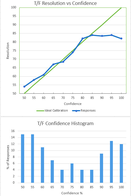
The nature of overconfidence is seen in the plot of resolution (response correctness) vs. confidence. Our confidence roughly matches our accuracy up to the point where confidence is moderately high, around 85%. After this, increased confidence occurs with no increase in accuracy. At at 100% confidence level, respondents were, on average, less correct than they were at 95% confidence. Much of that effect stemmed from the one “trick” question in each group of 10; people tend to be confident but wrong about hot topics with high media coverage.
The distribution of confidence values expressed by participants was nominally bimodal. People expressed very high or very low confidence about the accuracy of their answers. The slight bump in confidence at 75% is likely an artifact of the test methodology. The default value of the confidence slider (website user interface element) was 75%. On clicking the Submit button, users were warned if most of their responses specified the default value, but an acquiescence effect appears to have present anyway. In Superforecasters Philip Tetlock observed that many people seem to have a “three settings” (yes, no, maybe) mindset about matters of probability. That could also explain the slight peak at 75%.
I’ve been using a similar approach to confidence calibration in group decision settings for the past three decades. I learned it from a DoD publication by Sarah Lichtenstein and Baruch Fischhoff while working on the Midgetman Small Intercontinental Ballistic Missile program in the mid 1980s. Doug Hubbard teaches a similar approach in his book The Failure of Risk Management. In my experience with diverse groups contributing to risk analysis, where group decisions about likelihood of uncertain events are needed, an hour of training using similar tools yields impressive improvements in calibration as measured above.
Risk Neutrality and Corporate Risk Frameworks
Posted by Bill Storage in Uncategorized on October 27, 2020
Wikipedia describes risk-neutrality in these terms: “A risk neutral party’s decisions are not affected by the degree of uncertainty in a set of outcomes, so a risk-neutral party is indifferent between choices with equal expected payoffs even if one choice is riskier”
While a useful definition, it doesn’t really help us get to the bottom of things since we don’t all remotely agree on what “riskier” means. Sometimes, by “risk,” we mean an unwanted event: “falling asleep at the wheel is one of the biggest risks of nighttime driving.” Sometimes we equate “risk” with the probability of the unwanted event: “the risk of losing in roulette is 35 out of 36. Sometimes we mean the statistical expectation. And so on.
When the term “risk” is used in technical discussions, most people understand it to involve some combination of the likelihood (probability) and cost (loss value) of an unwanted event.
We can compare both the likelihoods and the costs of different risks, but deciding which is “riskier” using a one-dimensional range (i.e., higher vs. lower) requires a scalar calculus of risk. If risk is a combination of probability and severity of an unwanted outcome, riskier might equate to a larger value of the arithmetic product of the relevant probability (a dimensionless number between zero and one) and severity, measured in dollars.
But defining risk as such a scalar (area under the curve, therefore one dimensional) value is a big step, one that most analyses of human behavior suggests is not an accurate representation of how we perceive risk. It implies risk-neutrality.
Most people agree, as Wikipedia states, that a risk-neutral party’s decisions are not affected by the degree of uncertainty in a set of outcomes. On that view, a risk-neutral party is indifferent between all choices having equal expected payoffs.
Under this definition, if risk-neutral, you would have no basis for preferring any of the following four choices over another:
1) a 50% chance of winning $100.00
2) An unconditional award of $50.
3) A 0.01% chance of winning $500,000.00
4) A 90% chance of winning $55.56.
If risk-averse, you’d prefer choices 2 or 4. If risk-seeking, you’d prefer 1 or 3.
Now let’s imagine, instead of potential winnings, an assortment of possible unwanted events, termed hazards in engineering, for which we know, or believe we know, the probability numbers. One example would be to simply turn the above gains into losses:
1) a 50% chance of losing $100.00
2) An unconditional payment of $50.
3) A 0.01% chance of losing $500,000.00
4) A 90% chance of losing $55.56.
In this example, there are four different hazards. Many argue that rational analysis of risk entails quantification of hazard severities, independent of whether their probabilities are quantified. Above we have four risks, all having the same $50 expected value (cost), labeled 1 through 4. Whether those four risks can be considered equal depends on whether you are risk-neutral.
If forced to accept one of the four risks, a risk-neutral person would be indifferent to the choice; a risk seeker might choose risk 3, etc. Banks are often found to be risk-averse. That is, they will pay more to prevent risk 3 than to prevent risk 4, even though they have the same expected value. Viewed differently, banks often pay much more to prevent one occurrence of hazard 3 (cost = $500,000) than to prevent 9000 occurrences of hazard 4 (cost = $500,000).
Businesses compare risks to decide whether to reduce their likelihood, to buy insurance, or to take other actions. They often use a heat-map approach (sometimes called risk registers) to visualize risks. Heat maps plot probability vs severity and view any particular risk’s riskiness as the area of the rectangle formed by the axes and the point on the map representing that risk. Lines of constant risk therefore look like y = 1 / x. To be precise, they take the form of y = a/x where a represents a constant number of dollars called the expected value (or mathematical expectation or first moment) depending on area of study.
By plotting the four probability-cost vector values (coordinates) of the above four risks, we see that they all fall on the same line of constant risk. A sample curve of this form, representing a line of constant risk appears below on the left.
In my example above, the four points (50% chance of losing $100, etc.) have a large range of probabilities. Plotting these actual values on a simple grid isn’t very informative because the data points are far from the part of the plotted curve where the bend is visible (plot below on the right).
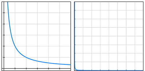
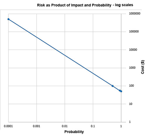
Students of high-school algebra know the fix for the problem of graphing data of this sort (monomials) is to use log paper. By plotting equations of the form described above using logarithmic scales for both axes, we get a straight line, having data points that are visually compressed, thereby taming the large range of the data, as below.
The risk frameworks used in business take a different approach. Instead of plotting actual probability values and actual costs, they plot scores, say from one ten. Their reason for doing this is more likely to convert an opinion into a numerical value than to cluster data for easy visualization. Nevertheless, plotting scores – on linear, not logarithmic, scales – inadvertently clusters data, though the data might have lost something in the translation to scores in the range of 1 to 10. In heat maps, this compression of data has the undesirable psychological effect of implying much small ranges for the relevant probability values and costs of the risks under study.
A rich example of this effect is seen in the 2002 PmBok (Project Management Body of Knowledge) published by the Project Management Institute. It assigns a score (which it curiously calls a rank) of 10 for probability values in the range of 0.5, a score of 9 for p=0.3, and a score of 8 for p=0.15. It should be obvious to most having a background in quantified risk that differentiating failure probabilities of .5, .3, and .15 is pointless and indicative of bogus precision, whether the probability is drawn from observed frequencies or from subjectivist/Bayesian-belief methods.
The methodological problem described above exists in frameworks that are implicitly risk-neutral. The real problem with the implicit risk-neutrality of risk frameworks is that very few of us – individuals or corporations – are risk-neutral. And no framework is right to tell us that we should be. Saying that it is somehow rational to be risk-neutral pushes the definition of rationality too far.
As proud king of a small distant planet of 10 million souls, you face an approaching comet that, on impact, will kill one million (10%) in your otherwise peaceful world. Your scientists and engineers rush to build a comet-killer nuclear rocket. The untested device has a 90% chance of destroying the comet but a 10% chance of exploding on launch thereby killing everyone on your planet. Do you launch the comet-killer, knowing that a possible outcome is total extinction? Or do you sit by and watch one million die from a preventable disaster? Your risk managers see two choices of equal riskiness: 100% chance of losing one million and a 10% chance of losing 10 million. The expected value is one million lives in both cases. But in that 10% chance of losing 10 million, there is no second chance. It’s an existential risk.
If these two choices seem somehow different, you are not risk-neutral. If you’re tempted to leave problems like this in the capable hands of ethicists, good for you. But unaware boards of directors have left analogous dilemmas in the incapable hands of simplistic and simple-minded risk frameworks.
The risk-neutrality embedded in risk frameworks is a subtle and pernicious case of Hume’s Guillotine – an inference from “is” to “ought” concealed within a fact-heavy argument. No amount of data, whether measured frequencies or subjective probability estimates, whether historical expenses or projected costs, even if recorded as PmBok’s scores and ranks, can justify risk-neutrality to parties who are not risk-neutral. So why is it embed it in the frameworks our leading companies pay good money for?
The Dose Makes the Poison
Posted by Bill Storage in Uncategorized on October 19, 2020
Toxicity is binary in California. Or so says its governor and most of its residents.
Governor Newsom, who believes in science, recently signed legislation making California the first state to ban 24 toxic chemicals in cosmetics.
The governor’s office states “AB 2762 bans 24 toxic chemicals in cosmetics, which are linked to negative long-term health impacts especially for women and children.”
The “which” in that statement is a nonrestrictive pronoun, and the comma preceding it makes the meaning clear. The sentence says that all toxic chemicals are linked to health impacts and that AB 2762 bans 24 of them – as opposed to saying 24 chemicals that are linked to health effects are banned. One need not be a grammarian or George Orwell to get the drift.
California continues down the chemophobic path, established in the 1970s, of viewing all toxicity through the beloved linear no-threshold lens. That lens has served gullible Californians well since the 1974, when the Sierra Club, which had until then supported nuclear power as “one of the chief long-term hopes for conservation,” teamed up with the likes of Gov. Jerry Brown (1975-83, 2011-19) and William Newsom – Gavin’s dad, investment manager for Getty Oil – to scare the crap out of science-illiterate Californians about nuclear power.

That fear-mongering enlisted Ralph Nadar, Paul Ehrlich and other leading Malthusians, rock stars, oil millionaires and overnight-converted environmentalists. It taught that nuclear plants could explode like atom bombs, and that anything connected to nuclear power was toxic – in any dose. At the same time Governor Brown, whose father had deep oil ties, found that new fossil fuel plants could be built “without causing environmental damage.” The Sierra Club agreed, and secretly took barrels of cash from fossil fuel companies for the next four decades – $25M in 2007 from subsidiaries of, and people connected to, Chesapeake Energy.
What worked for nuclear also works for chemicals. “Toxic chemicals have no place in products that are marketed for our faces and our bodies,” said First Partner Jennifer Siebel Newsom in response to the recent cosmetics ruling. Jennifer may be unaware that the total amount of phthalates in the banned zipper tabs would yield very low exposure indeed.
Chemicals cause cancer, especially in California, where you cannot enter a parking garage, nursery, or Starbucks without reading a notice that the place can “expose you to chemicals known to the State of California to cause birth defects.” California’s litigator-lobbied legislators authored Proposition 65 in a way that encourages citizens to rat on violators, the “citizen enforcers” receiving 25% of any penalties assessed by the court. The proposition lead chemophobes to understand that anything “linked to cancer” causes cancer. It exaggerates theoretical cancer risks stymying the ability of the science-ignorant educated class to make reasonable choices about actual risks like measles and fungus.
California’s linear no-threshold conception of chemical carcinogens actually started in 1962 with Rachel Carson’s Silent Spring, the book that stopped DDT use, saving all the birds, with the minor side effect of letting millions of Africans die of malaria who would have survived (1, 2, 3) had DDT use continued.
But ending DDT didn’t save the birds, because DDT wasn’t the cause of US bird death as Carson reported, because the bird death at the center of her impassioned plea never happened. This has been shown by many subsequent studies; and Carson, in her work at Fish and Wildlife Service and through her participation in Audubon bird counts, certainly had access to data showing that the eagle population doubled, and robin, catbird, and dove counts had increased by 500% between the time DDT was introduced and her eloquence, passionate telling of the demise of the days that once “throbbed with the dawn chorus of robins, catbirds, and doves.”
Carson also said that increasing numbers of children were suffering from leukemia, birth defects and cancer, and of “unexplained deaths,” and that “women were increasingly unfertile.” Carson was wrong about increasing rates of these human maladies, and she lied about the bird populations. Light on science, Carson was heavy on influence: “Many real communities have already suffered.”
In 1969 the Environmental Defense Fund demanded a hearing on DDT. Lasting eight months, the examiner’s verdict concluded DDT was not mutagenic or teratogenic. No cancer, no birth defects. In found no “deleterious effect on freshwater fish, estuarine organisms, wild birds or other wildlife.”
William Ruckleshaus, first director of the EPA didn’t attend the hearings or read the transcript. Pandering to the mob, he chose to ban DDT in the US anyway. It was replaced by more harmful pesticides in the US and the rest of the world. In praising Ruckleshaus, who died last year, NPR, the NY Times and the Puget Sound Institute described his having a “preponderance of evidence” of DDT’s damage, never mentioning the verdict of that hearing.
When Al Gore took up the cause of climate, he heaped praise on Carson, calling her book “thoroughly researched.” Al’s research on Carson seems of equal depth to Carson’s research on birds and cancer. But his passion and unintended harm have certainly exceeded hers. A civilization relying on the low-energy-density renewables Gore advocates will consume somewhere between 100 and 1000 times more space for food and energy than we consume at present.
California’s fallacious appeal to naturalism regarding chemicals also echoes Carson’s, and that of her mentor, Wilhelm Hueper, who dedicated himself to the idea that cancer stemmed from synthetic chemicals. This is still overwhelmingly the sentiment of Californians, despite the fact that the smoking-tar-cancer link now seems a bit of a fluke. That is, we expected the link between other “carcinogens” and cancer to be as clear as the link between smoking and cancer. It is not remotely. As George Johnson, author of The Cancer Chronicles, wrote, “as epidemiology marches on, the link between cancer and carcinogen seems ever fuzzier” (re Tomasetti on somatic mutations). Carson’s mentor Hueper, incidentally, always denied that smoking caused cancer, insisting toxic chemicals released by industry caused lung cancer.
This brings us back to the linear no-threshold concept. If a thing kills mice in high doses, then any dose to humans is harmful – in California. And that’s accepting that what happens in mice happens in humans, but mice lie and monkeys exaggerate. Outside California, most people are at least aware of certain hormetic effects (U-shaped dose-response curve). Small amounts of Vitamin C prevent scurvy; large amounts cause nephrolithiasis. Small amounts of penicillin promote bacteria growth; large amount kill them. There is even evidence of biopositive effects from low-dose radiation, suggesting that 6000 millirems a year might be best for your health. The current lower-than-baseline levels of cancers in 10,000 residents of Taiwan accidentally exposed to radiation-contaminated steel, in doses ranging from 13 to 160 mSv/yr for ten years starting in 1982 is a fascinating case.
Radiation aside, perpetuating a linear no-threshold conception of toxicity in the science-illiterate electorate for political reasons is deplorable, as is the educational system that produces degreed adults who are utterly science-illiterate – but “believe in science” and expect their government to dispense it responsibly. The Renaissance physician Paracelsus knew better half a millennium ago when he suggested that that substances poisonous in large doses may be curative in small ones, writing that “the dose makes the poison.”
To demonstrate chemophobia in 2003, Penn Jillette and assistant effortlessly convinced people in a beach community, one after another, to sign a petition to ban dihydrogen monoxide (H2O). Water is of course toxic in high doses, causing hyponatremia, seizures and brain damage. But I don’t think Paracelsus would have signed the petition.

The Prosecutor’s Fallacy Illustrated
Posted by Bill Storage in Probability and Risk on May 7, 2020
“The first thing we do, let’s kill all the lawyers.” – Shakespeare, Henry VI, Part 2, Act IV
My last post discussed the failure of most physicians to infer the chance a patient has the disease given a positive test result where both the frequency of the disease in the population and the accuracy of the diagnostic test are known. The probability that the patient has the disease can be hundreds or thousands of times lower than the accuracy of the test. The problem in reasoning that leads us to confuse these very different likelihoods is one of several errors in logic commonly called the prosecutor’s fallacy. The important concept is conditional probability. By that we mean simply that the probability of x has a value and that the probability of x given that y is true has a different value. The shorthand for probability of x is p(x) and the shorthand for probability of x given y is p(x|y).
“Punching, pushing and slapping is a prelude to murder,” said prosecutor Scott Gordon during the trial of OJ Simpson for the murder of Nicole Brown. Alan Dershowitz countered with the argument that the probability of domestic violence leading to murder was very remote. Dershowitz (not prosecutor but defense advisor in this case) was right, technically speaking. But he was either as ignorant as the physicians interpreting the lab results or was giving a dishonest argument, or possibly both. The relevant probability was not the likelihood of murder given domestic violence, it was the likelihood of murder given domestic violence and murder. “The courtroom oath – to tell the truth, the whole truth and nothing but the truth – is applicable only to witnesses,” said Dershowitz in The Best Defense. In Innumeracy: Mathematical Illiteracy and Its Consequences. John Allen Paulos called Dershowitz’s point “astonishingly irrelevant,” noting that utter ignorance about probability and risk “plagues far too many otherwise knowledgeable citizens.” Indeed.
The doctors’ mistake in my previous post was confusing
P(positive test result) vs.
P(disease | positive test result)
Dershowitz’s argument confused
P(husband killed wife | husband battered wife) vs.
P(husband killed wife | husband battered wife | wife was killed)
In Reckoning With Risk, Gerd Gigerenzer gave a 90% value for the latter Simpson probability. What Dershowitz cited was the former, which we can estimate at 0.1%, given a wife-battery rate of one in ten, and wife-murder rate of one per hundred thousand. So, contrary to what Dershowitz implied, prior battery is a strong indicator of guilt when a wife has been murdered.
As mentioned in the previous post, the relevant mathematical rule does not involve advanced math. It’s a simple equation due to Pierre-Simon Laplace, known, oddly, as Bayes’ Theorem:
P(A|B) = P(B|A) * P(A) / P(B)
If we label the hypothesis (patient has disease) as D and the test data as T, the useful form of Bayes’ Theorem is
P(D|T) = P(T|D) P(D) / P(T) where P(T) is the sum of probabilities of positive results, e.g.,
P(T) = P(T|D) * P(D) + P(T | not D) * P(not D) [using “not D” to mean “not diseased”]
Cascells’ phrasing of his Harvard quiz was as follows: “If a test to detect a disease whose prevalence is 1 out of 1,000 has a false positive rate of 5 percent, what is the chance that a person found to have a positive result actually has the disease?”
Plugging in the numbers from the Cascells experiment (with the parameters Cascells provided shown below in bold and the correct answer in green):
- P(D) is the disease frequency = 0.001 [ 1 per 1000 in population ] therefore:
- P(not D) is 1 – P(D) = 0.999
- P(T | not D) = 5% = 0.05 [ false positive rate also 5%] therefore:
- P(T | D) = 95% = 0.95 [ i.e, the false negative rate is 5% ]
Substituting:
P(T) = .95 * .001 + .999 * .05 = 0.0509 ≈ 5.1% [ total probability of a positive test ]
P(D|T) = .95 * .001 / .0509 = .0019 ≈ 2% [ probability that patient has disease, given a positive test result ]
Voila.
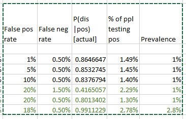
I hope this seeing is believing illustration of Cascells’ experiment drives the point home for those still uneasy with equations. I used Cascells’ rates and a population of 100,000 to avoid dealing with fractional people:
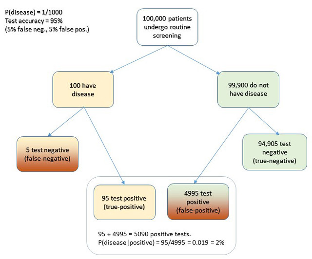
Extra credit: how exactly does this apply to Covid, news junkies?
Edit 5/21/20. An astute reader called me on an inaccuracy in the diagram. I used an approximation, without identifying it. P = r1/r2 is a cheat for P = 1 – Exp(- r1/r2). The approximation is more intuitive, though technically wrong. It’s a good cheat, for P values less that 10%.
Note 5/22/20. In response to questions about how this sort of thinking bears on coronavirus testing -what test results say about prevalence – consider this. We really have one equation in 3 unknowns here: false positive rate, false negative rate, and prevalence in population. A quick Excel variations study using false positive rates from 1 to 20% and false neg rates from 1 to 3 percent, based on a quick web search for proposed sensitivity/specificity for the Covid tests is revealing. Taking the low side of the raw positive rates from the published data (1 – 3%) results in projected prevalence roughly equal to the raw positive rates. I.e., the false positives and false negatives happen to roughly wash out in this case. That also leaves P(d|t) in the range of a few percent.
Innumeracy and Overconfidence in Medical Training
Posted by Bill Storage in History of Science on May 4, 2020
Most medical doctors, having ten or more years of education, can’t do simple statistics calculations that they were surely able to do, at least for a week or so, as college freshmen. Their education has let them down, along with us, their patients. That education leaves many doctors unquestioning, unscientific, and terribly overconfident.
A disturbing lack of doubt has plagued medicine for thousands of years. Galen, at the time of Marcus Aurelius, wrote, “It is I, and I alone, who has revealed the true path of medicine.” Galen disdained empiricism. Why bother with experiments and observations when you own the truth. Galen’s scientific reasoning sounds oddly similar to modern junk science armed with abundant confirming evidence but no interest in falsification. Galen had plenty of confirming evidence: “All who drink of this treatment recover in a short time, except those whom it does not help, who all die. It is obvious, therefore, that it fails only in incurable cases.”
Galen was still at work 1500 years later when Voltaire wrote that the art of medicine consisted of entertaining the patient while nature takes its course. One of Voltaire’s novels also described a patient who had survived despite the best efforts of his doctors. Galen was around when George Washington died after five pints of bloodletting, a practice promoted up to the early 1900s by prominent physicians like Austin Flint.
 But surely medicine was mostly scientific by the 1900s, right? Actually, 20th century medicine was dragged kicking and screaming to scientific methodology. In the early 1900’s Ernest Amory Codman of Massachusetts General proposed keeping track of patients and rating hospitals according to patient outcome. He suggested that a doctor’s reputation and social status were poor measures of a patient’s chance of survival. He wanted the track records of doctors and hospitals to be made public, allowing healthcare consumers to choose suppliers based on statistics. For this, and for his harsh criticism of those who scoffed at his ideas, Codman was tossed out of Mass General, lost his post at Harvard, and was suspended from the Massachusetts Medical Society. Public outcry brought Codman back into medicine, and much of his “end results system” was put in place.
20th century medicine also fought hard against the concept of controlled trials. Austin Bradford Hill introduced the concept to medicine in the mid 1920s. But in the mid 1950s Dr. Archie Cochrane was still fighting valiantly against what he called the God Complex in medicine, which was basically the ghost of Galen; no one should question the authority of a physician. Cochrane wrote that far too much of medicine lacked any semblance of scientific validation and knowing what treatments actually worked. He wrote that the medical establishment was hostile the idea of controlled trials. Cochrane fought this into the 1970s, authoring Effectiveness and Efficiency: Random Reflections on Health Services in 1972.
Doctors aren’t naturally arrogant. The God Complex is passed passed along during the long years of an MD’s education and internship. That education includes rights of passage in an old boys’ club that thinks sleep deprivation builds character in interns, and that female med students should make tea for the boys. Once on the other side, tolerance of archaic norms in the MD culture seems less offensive to the inductee, who comes to accept the system. And the business of medicine, the way it’s regulated, and its control by insurance firms, pushes MDs to view patients as a job to be done cost-effectively. Medical arrogance is in a sense encouraged by recovering patients who might see doctors as savior figures.
As Daniel Kahneman wrote, “generally, it is considered a weakness and a sign of vulnerability for clinicians to appear unsure.” Medical overconfidence is encouraged by patients’ preference for doctors who communicate certainties, even when uncertainty stems from technological limitations, not from doctors’ subject knowledge. MDs should be made conscious of such dynamics and strive to resist inflating their self importance. As Allan Berger wrote in Academic Medicine in 2002, “we are but an instrument of healing, not its source.”
Many in medical education are aware of these issues. The calls for medical education reform – both content and methodology – are desperate, but they are eerily similar to those found in a 1924 JAMA article, Current Criticism of Medical Education.
Covid19 exemplifies the aspect of medical education I find most vile. Doctors can’t do elementary statistics and probability, and their cultural overconfidence renders them unaware of how critically they need that missing skill.
A 1978 study, brought to the mainstream by psychologists like Kahnemann and Tversky, showed how few doctors know the meaning of a positive diagnostic test result. More specifically, they’re ignorant of the relationship between the sensitivity and specificity (true positive and true negative rates) of a test and the probability that a patient who tested positive has the disease. This lack of knowledge has real consequences In certain situations, particularly when the base rate of the disease in a population is low. The resulting probability judgements can be wrong by factors of hundreds or thousands.
In the 1978 study (Cascells et. al.) doctors and medical students at Harvard teaching hospitals were given a diagnostic challenge. “If a test to detect a disease whose prevalence is 1 out of 1,000 has a false positive rate of 5 percent, what is the chance that a person found to have a positive result actually has the disease?” As described, the true positive rate of the diagnostic test is 95%. This is a classic conditional-probability quiz from the second week of a probability class. Being right requires a), knowing Bayes Theorem, and b), being able to multiply and divide. Not being confidently wrong requires only one thing: scientific humility – the realization that all you know might be less than all there is to know. The correct answer is 2% – there’s a 2% likelihood the patient has the disease. The most common response, by far, in the 1978 study was 95%, which is wrong by 4750%. Only 18% of doctors and med students gave the correct response. The study’s authors observed that in the group tested, “formal decision analysis was almost entirely unknown and even common-sense reasoning about the interpretation of laboratory data was uncommon.”
As mentioned above, this story was heavily publicized in the 80s. It was widely discussed by engineering teams, reliability departments, quality assurance groups and math departments. But did it impact medical curricula, problem-based learning, diagnostics training, or any other aspect of the way med students were taught? One might have thought yes, if for no reason than to avoid criticism by less prestigious professions having either the relevant knowledge of probability or the epistemic humility to recognize that the right answer might be far different from the obvious one.
Similar surveys were done in 1984 (David M Eddy) and in 2003 (Kahan, Paltiel) with similar results. In 2013, Manrai and Bhatia repeated Cascells’ 1978 survey with the exact same wording, getting trivially better results. 23% answered correctly. They suggesting that medical education “could benefit from increased focus on statistical inference.” That was 35 years after Cascells, during which, the phenomenon was popularized by the likes of Daniel Kahneman, from the perspective of base-rate neglect, by Philip Tetlock, from the perspective of overconfidence in forecasting, and by David Epstein, from the perspective of the tyranny of specialization.
Over the past decade, I’ve asked the Cascells question to doctors I’ve known or met, where I didn’t think it would get me thrown out of the office or booted from a party. My results were somewhat worse. Of about 50 MDs, four answered correctly or were aware that they’d need to look up the formula but knew that it was much less than 95%. One was an optometrist, one a career ER doc, one an allergist-immunologist, and one a female surgeon – all over 50 years old, incidentally.
Despite the efforts of a few radicals in the Accreditation Council for Graduate Medical Education and some post-Flexnerian reformers, medical education remains, as Jonathan Bush points out in Tell Me Where It Hurts, basically a 2000 year old subject-based and lecture-based model developed at a time when only the instructor had access to a book. Despite those reformers, basic science has actually diminished in recent decades, leaving many physicians with less of a grasp of scientific methodology than that held by Ernest Codman in 1915. Medical curriculum guardians, for the love of God, get over your stodgy selves and replace the calculus badge with applied probability and statistical inference from diagnostics. Place it later in the curriculum later than pre-med, and weave it into some of that flipped-classroom, problem-based learning you advertise.
55 Saves Lives
Posted by Bill Storage in Systems Engineering on April 15, 2020
Congress and Richard Nixon had no intention to pull a bait-and-switch when the enacted the National Maximum Speed Law (NMSL) on Jan. 2, 1974. The emergency response to an embargo, NMSL (Public Law 93-239), specified that it was “an act to conserve energy on the Nation’s highways.” Conservation, in this context, meant reducing oil consumption to prevent the embargo proclaimed by the Organization of Arab Petroleum Exporting in October 1973 from seriously impacting American production or causing a shortage of oil then used for domestic heating. There was a precedent. A national speed limit had been imposed for the same reasons during World War II.
By the summer of 1974 the threat of oil shortage was over. But unlike the case after the war, many government officials, gently nudged by auto insurance lobbies, argued that the reduced national speed limit would save tens of thousands of lives annually. Many drivers conspicuously displayed their allegiance to the cause with bumper stickers reminding us that “55 Saves Lives.” Bad poetry, you may say in hindsight, a sorry attempt at trochaic monometer. But times were desperate and less enlightened drivers had to be brought onboard. We were all in it together.
Over the next ten years, the NMSL became a major boon to jurisdictions crossed by interstate highways, some earning over 80% of their revenues from speeding fines. Studies reached conflicting findings over whether the NMSL had saved fuel or lives. The former seems undeniable at first glance, but the resulting increased congestion caused frequent brake/stop/accelerate effects in cities, and the acceleration phase is a gas guzzler. Those familiar with fluid mechanics note that the traffic capacity of a highway is proportional to the speed driven on it. Some analyses showed decreased fuel efficiency (net miles per gallon). The most generous analyses reported a less than 1% decrease in consumption.
No one could argue that 55 mph collisions were more dangerous than 70 mph collisions. But some drivers, particularly in the west, felt betrayed after being told that the NMSL was an emergency measure (”during periods of current and imminent fuel shortages”) to save oil and then finding it would persist indefinitely for a new reason, to save lives. Hicks and greasy trucker pawns of corporate fat cats, my science teachers said of those arguing to repeal the NMSL.
The matter was increasingly argued over the next twelve years. The states’ rights issue was raised. Some remembered that speed limits had originally been set by a democratic 85% rule. The 85th percentile speed of drivers on an unposted highway became the limit for that road. Auto fatality rates had dropped since 1974, and everyone had their theories as to why. A case was eventually made for an experimental increase to 65 mph, approved by Congress in December 1987. The insurance lobby predicted carnage. Ralph Nader announced that “history will never forgive Congress for this assault on the sanctity of human life.”
Between 1987 and 1995, 40 states moved to the 65 limit. Auto fatality rates continued to decrease as they had done between 1973 and 1987, during which time some radical theorists had argued that the sudden drop in fatality rate in early 1974 had been a statistical blip regressed to the mean a year later and that better cars and seat belt usage accounted for the decreased mortality. Before 1987, those arguments were commonly understood to be mere rationalizations.
In December 1995, more than twenty years after being enacted, Congress finally undid the NMSL completely. States had the authority to set speed limits. An unexpected result of increasing speed limits to 75 mph in some western states was that, as revealed by unmanned radar, the number of vehicles driving above 80 mph dropped by 85% compared to when the speed limit was 65.
From a systems-theory perspective, it’s clear that the highway transportation network is a complex phenomenon, one resistant to being modeled through facile conjecture about causes and effects, naive assumptions about incentives and human behavior, and ivory-tower analytics.
The Covid Megatilt
Posted by Bill Storage in Uncategorized on April 3, 2020
Playing poker online is far more addictive than gambling in a casino. Online poker, and other online gambling that involves a lot of skill, is engineered for addiction. Online poker allows multiple simultaneous tables. Laptops, tablets, and mobile phones provide faster play than in casinos. Setup time, for an efficient addict, can be seconds per game. Better still, you can rapidly switch between different online games to get just enough variety to eliminate any opportunity for boredom that has not been engineered out of the gaming experience. Completing a hand of Texas Holdem in 45 seconds online increases your chances of fast wins, fast losses, and addiction.
Tilt is what poker players call it when a particular run of bad luck, an opponent’s skill, or that same opponent’s obnoxious communications put you into a mental state where you’re playing emotionally and not rationally. Anger, disgust, frustration and distress is precipitated by bad beats, bluffs gone awry, a run of dead cards, losing to a lower ranked opponent, fatigue, or letting the opponent’s offensive demeanor get under your skin. 
Tilt is so important to online poker that many products and commitment devices have emerged to deal with it. Tilt Breaker provides services like monitoring your performance to detect fatigue and automated stop-loss protection that restricts betting or table count after a run of losses.
A few years back, some friends and I demonstrated biometric tilt detection using inexpensive heart rate sensors. We used machine learning with principal dynamic modes (PDM) analysis running in a mobile app to predict sympathetic (stress-inducing, cortisol, epinephrine) and parasympathetic (relaxation, oxytocin) nervous system activity. We then differentiated mental and physical stress using the mobile phone’s accelerometer and location functions. We could ring an alarm to force a player to face being at risk of tilt or ragequit, even if he was ignoring the obvious physical cues. Maybe it’s time to repurpose this technology.
In past crises, the flow of bad news and peer communications were limited by technology. You could not scroll through radio programs or scan through TV shows. You could click between the three news stations, and then you were stuck. Now you can consume all of what could be home work and family time with up to the minute Covid death tolls while blasting your former friends on Twitter and Facebook for their appalling politicization of the crisis.
You yourself are of course innocent of that sort of politicizing. As a seasoned poker player, you know that the more you let emotions take control your game, the farther your judgments will stray from rational ones.
Still yet, what kind of utter moron could think that the whole response to Covid is a media hoax? Or that none of it is.

Recent Comments