Posts Tagged probability and statistics
Statistical Reasoning in Healthcare: Lessons from Covid-19
Posted by Bill Storage in History of Science, Philosophy of Science, Probability and Risk on May 6, 2025
For centuries, medicine has navigated the tension between science and uncertainty. The Covid pandemic exposed this dynamic vividly, revealing both the limits and possibilities of statistical reasoning. From diagnostic errors to vaccine communication, the crisis showed that statistics is not just a technical skill but a philosophical challenge, shaping what counts as knowledge, how certainty is conveyed, and who society trusts.
Historical Blind Spot
Medicine’s struggle with uncertainty has deep roots. In antiquity, Galen’s reliance on reasoning over empirical testing set a precedent for overconfidence insulated by circular logic. If his treatments failed, it was because the patient was incurable. Enlightenment physicians, like those who bled George Washington to death, perpetuated this resistance to scrutiny. Voltaire wrote, “The art of medicine consists in amusing the patient while nature cures the disease.” The scientific revolution and the Enlightenment inverted Galen’s hierarchy, yet the importance of that reversal is often neglected, even by practitioners. Even in the 20th century, pioneers like Ernest Codman faced ostracism for advocating outcome tracking, highlighting a medical culture that prized prestige over evidence. While evidence-based practice has since gained traction, a statistical blind spot persists, rooted in training and tradition.
The Statistical Challenge
Physicians often struggle with probabilistic reasoning, as shown in a 1978 Harvard study where only 18% correctly applied Bayes’ Theorem to a diagnostic test scenario (a disease with 1/1,000 prevalence and a 5% false positive rate yields a ~2% chance of disease given a positive test). A 2013 follow-up showed marginal improvement (23% correct). Medical education, which prioritizes biochemistry over probability, is partly to blame. Abusive lawsuits, cultural pressures for decisiveness, and patient demands for certainty further discourage embracing doubt, as Daniel Kahneman’s work on overconfidence suggests.
Neil Ferguson and the Authority of Statistical Models
Epidemiologist Neil Ferguson and his team at Imperial College London produced a model in March 2020 predicting up to 500,000 UK deaths without intervention. The US figure could top 2 million. These weren’t forecasts in the strict sense but scenario models, conditional on various assumptions about disease spread and response.
Ferguson’s model was extraordinarily influential, shifting the UK and US from containment to lockdown strategies. It also drew criticism for opaque code, unverified assumptions, and the sheer weight of its political influence. His eventual resignation from the UK’s Scientific Advisory Group for Emergencies (SAGE) over a personal lockdown violation further politicized the science.
From the perspective of history of science, Ferguson’s case raises critical questions: When is a model scientific enough to guide policy? How do we weigh expert uncertainty under crisis? Ferguson’s case shows that modeling straddles a line between science and advocacy. It is, in Kuhnian terms, value-laden theory.
The Pandemic as a Pedagogical Mirror
The pandemic was a crucible for statistical reasoning. Successes included the clear communication of mRNA vaccine efficacy (95% relative risk reduction) and data-driven ICU triage using the SOFA score, though both had limitations. Failures were stark: clinicians misread PCR test results by ignoring pre-test probability, echoing the Harvard study’s findings, while policymakers fixated on case counts over deaths per capita. The “6-foot rule,” based on outdated droplet models, persisted despite disconfirming evidence, reflecting resistance to updating models, inability to apply statistical insights, and institutional inertia. Specifics of these issues are revealing.
Mostly Positive Examples:
- Risk Communication in Vaccine Trials (1)
The early mRNA vaccine announcements in 2020 offered clear statistical framing by emphasizing a 95% relative risk reduction in symptomatic COVID-19 for vaccinated individuals compared to placebo, sidelining raw case counts for a punchy headline. While clearer than many public health campaigns, this focus omitted absolute risk reduction and uncertainties about asymptomatic spread, falling short of the full precision needed to avoid misinterpretation. - Clinical Triage via Quantitative Models (2)
During peak ICU shortages, hospitals adopted the SOFA score, originally a tool for assessing organ dysfunction, to guide resource allocation with a semi-objective, data-driven approach. While an improvement over ad hoc clinical judgment, SOFA faced challenges like inconsistent application and biases that disadvantaged older or chronically ill patients, limiting its ability to achieve fully equitable triage. - Wastewater Epidemiology (3)
Public health researchers used viral RNA in wastewater to monitor community spread, reducing the sampling biases of clinical testing. This statistical surveillance, conducted outside clinics, offered high public health relevance but faced biases and interpretive challenges that tempered its precision.
Mostly Negative Examples:
- Misinterpretation of Test Results (4)
Early in the COVID-19 pandemic, many clinicians and media figures misunderstood diagnostic test accuracy, misreading PCR and antigen test results by overlooking pre-test probability. This caused false reassurance or unwarranted alarm, though some experts mitigated errors with Bayesian reasoning. This was precisely the type of mistake highlighted in the Harvard study decades earlier. - Cases vs. Deaths (5)
One of the most persistent statistical missteps during the pandemic was the policy focus on case counts, devoid of context. Case numbers ballooned or dipped not only due to viral spread but due to shifts in testing volume, availability, and policies. COVID deaths per capita rather than case count would have served as a more stable measure of public health impact. Infection fatality rates would have been better still. - Shifting Guidelines and Aerosol Transmission (6)
The “6-foot rule” was based on outdated models of droplet transmission. When evidence of aerosol spread emerged, guidance failed to adapt. Critics pointed out the statistical conservatism in risk modeling, its impact on mental health and the economy. Institutional inertia and politics prevented vital course corrections.
(I’ll defend these six examples in another post.)
A Philosophical Reckoning
Statistical reasoning is not just a mathematical tool – it’s a window into how science progresses, how it builds trust, and its special epistemic status. In Kuhnian terms, the pandemic exposed the fragility of our current normal science. We should expect methodological chaos and pluralism within medical knowledge-making. Science during COVID-19 was messy, iterative, and often uncertain – and that’s in some ways just how science works.
This doesn’t excuse failures in statistical reasoning. It suggests that training in medicine should not only include formal biostatistics, but also an eye toward history of science – so future clinicians understand the ways that doubt, revision, and context are intrinsic to knowledge.
A Path Forward
Medical education must evolve. First, integrate Bayesian philosophy into clinical training, using relatable case studies to teach probabilistic thinking. Second, foster epistemic humility, framing uncertainty as a strength rather than a flaw. Third, incorporate the history of science – figures like Codman and Cochrane – to contextualize medicine’s empirical evolution. These steps can equip physicians to navigate uncertainty and communicate it effectively.
Conclusion
Covid was a lesson in the fragility and potential of statistical reasoning. It revealed medicine’s statistical struggles while highlighting its capacity for progress. By training physicians to think probabilistically, embrace doubt, and learn from history, medicine can better manage uncertainty – not as a liability, but as a cornerstone of responsible science. As John Heilbron might say, medicine’s future depends not only on better data – but on better historical memory, and the nerve to rethink what counts as knowledge.
______
All who drink of this treatment recover in a short time, except those whom it does not help, all of whom die. It is obvious, therefore, that it fails only in incurable cases. – Galen
Risk Neutrality and Corporate Risk Frameworks
Posted by Bill Storage in Uncategorized on October 27, 2020
Wikipedia describes risk-neutrality in these terms: “A risk neutral party’s decisions are not affected by the degree of uncertainty in a set of outcomes, so a risk-neutral party is indifferent between choices with equal expected payoffs even if one choice is riskier”
While a useful definition, it doesn’t really help us get to the bottom of things since we don’t all remotely agree on what “riskier” means. Sometimes, by “risk,” we mean an unwanted event: “falling asleep at the wheel is one of the biggest risks of nighttime driving.” Sometimes we equate “risk” with the probability of the unwanted event: “the risk of losing in roulette is 35 out of 36. Sometimes we mean the statistical expectation. And so on.
When the term “risk” is used in technical discussions, most people understand it to involve some combination of the likelihood (probability) and cost (loss value) of an unwanted event.
We can compare both the likelihoods and the costs of different risks, but deciding which is “riskier” using a one-dimensional range (i.e., higher vs. lower) requires a scalar calculus of risk. If risk is a combination of probability and severity of an unwanted outcome, riskier might equate to a larger value of the arithmetic product of the relevant probability (a dimensionless number between zero and one) and severity, measured in dollars.
But defining risk as such a scalar (area under the curve, therefore one dimensional) value is a big step, one that most analyses of human behavior suggests is not an accurate representation of how we perceive risk. It implies risk-neutrality.
Most people agree, as Wikipedia states, that a risk-neutral party’s decisions are not affected by the degree of uncertainty in a set of outcomes. On that view, a risk-neutral party is indifferent between all choices having equal expected payoffs.
Under this definition, if risk-neutral, you would have no basis for preferring any of the following four choices over another:
1) a 50% chance of winning $100.00
2) An unconditional award of $50.
3) A 0.01% chance of winning $500,000.00
4) A 90% chance of winning $55.56.
If risk-averse, you’d prefer choices 2 or 4. If risk-seeking, you’d prefer 1 or 3.
Now let’s imagine, instead of potential winnings, an assortment of possible unwanted events, termed hazards in engineering, for which we know, or believe we know, the probability numbers. One example would be to simply turn the above gains into losses:
1) a 50% chance of losing $100.00
2) An unconditional payment of $50.
3) A 0.01% chance of losing $500,000.00
4) A 90% chance of losing $55.56.
In this example, there are four different hazards. Many argue that rational analysis of risk entails quantification of hazard severities, independent of whether their probabilities are quantified. Above we have four risks, all having the same $50 expected value (cost), labeled 1 through 4. Whether those four risks can be considered equal depends on whether you are risk-neutral.
If forced to accept one of the four risks, a risk-neutral person would be indifferent to the choice; a risk seeker might choose risk 3, etc. Banks are often found to be risk-averse. That is, they will pay more to prevent risk 3 than to prevent risk 4, even though they have the same expected value. Viewed differently, banks often pay much more to prevent one occurrence of hazard 3 (cost = $500,000) than to prevent 9000 occurrences of hazard 4 (cost = $500,000).
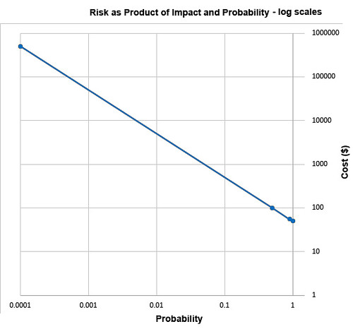
Businesses compare risks to decide whether to reduce their likelihood, to buy insurance, or to take other actions. They often use a heat-map approach (sometimes called risk registers) to visualize risks. Heat maps plot probability vs severity and view any particular risk’s riskiness as the area of the rectangle formed by the axes and the point on the map representing that risk. Lines of constant risk therefore look like y = 1 / x. To be precise, they take the form of y = a/x where a represents a constant number of dollars called the expected value (or mathematical expectation or first moment) depending on area of study.
By plotting the four probability-cost vector values (coordinates) of the above four risks, we see that they all fall on the same line of constant risk. A sample curve of this form, representing a line of constant risk appears below on the left.
In my example above, the four points (50% chance of losing $100, etc.) have a large range of probabilities. Plotting these actual values on a simple grid isn’t very informative because the data points are far from the part of the plotted curve where the bend is visible (plot below on the right).
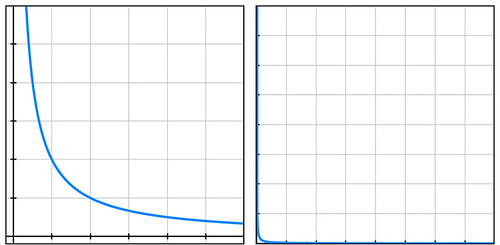
Students of high-school algebra know the fix for the problem of graphing data of this sort (monomials) is to use log paper. By plotting equations of the form described above using logarithmic scales for both axes, we get a straight line, having data points that are visually compressed, thereby taming the large range of the data, as below.
The risk frameworks used in business take a different approach. Instead of plotting actual probability values and actual costs, they plot scores, say from one ten. Their reason for doing this is more likely to convert an opinion into a numerical value than to cluster data for easy visualization. Nevertheless, plotting scores – on linear, not logarithmic, scales – inadvertently clusters data, though the data might have lost something in the translation to scores in the range of 1 to 10. In heat maps, this compression of data has the undesirable psychological effect of implying much small ranges for the relevant probability values and costs of the risks under study.
A rich example of this effect is seen in the 2002 PmBok (Project Management Body of Knowledge) published by the Project Management Institute. It assigns a score (which it curiously calls a rank) of 10 for probability values in the range of 0.5, a score of 9 for p=0.3, and a score of 8 for p=0.15. It should be obvious to most having a background in quantified risk that differentiating failure probabilities of .5, .3, and .15 is pointless and indicative of bogus precision, whether the probability is drawn from observed frequencies or from subjectivist/Bayesian-belief methods.
The methodological problem described above exists in frameworks that are implicitly risk-neutral. The real problem with the implicit risk-neutrality of risk frameworks is that very few of us – individuals or corporations – are risk-neutral. And no framework is right to tell us that we should be. Saying that it is somehow rational to be risk-neutral pushes the definition of rationality too far.
As proud king of a small distant planet of 10 million souls, you face an approaching comet that, on impact, will kill one million (10%) in your otherwise peaceful world. Your scientists and engineers rush to build a comet-killer nuclear rocket. The untested device has a 90% chance of destroying the comet but a 10% chance of exploding on launch thereby killing everyone on your planet. Do you launch the comet-killer, knowing that a possible outcome is total extinction? Or do you sit by and watch one million die from a preventable disaster? Your risk managers see two choices of equal riskiness: 100% chance of losing one million and a 10% chance of losing 10 million. The expected value is one million lives in both cases. But in that 10% chance of losing 10 million, there is no second chance. It’s an existential risk.
If these two choices seem somehow different, you are not risk-neutral. If you’re tempted to leave problems like this in the capable hands of ethicists, good for you. But unaware boards of directors have left analogous dilemmas in the incapable hands of simplistic and simple-minded risk frameworks.
The risk-neutrality embedded in risk frameworks is a subtle and pernicious case of Hume’s Guillotine – an inference from “is” to “ought” concealed within a fact-heavy argument. No amount of data, whether measured frequencies or subjective probability estimates, whether historical expenses or projected costs, even if recorded as PmBok’s scores and ranks, can justify risk-neutrality to parties who are not risk-neutral. So why is it embed it in the frameworks our leading companies pay good money for?
The Prosecutor’s Fallacy Illustrated
Posted by Bill Storage in Probability and Risk on May 7, 2020
“The first thing we do, let’s kill all the lawyers.” – Shakespeare, Henry VI, Part 2, Act IV
My last post discussed the failure of most physicians to infer the chance a patient has the disease given a positive test result where both the frequency of the disease in the population and the accuracy of the diagnostic test are known. The probability that the patient has the disease can be hundreds or thousands of times lower than the accuracy of the test. The problem in reasoning that leads us to confuse these very different likelihoods is one of several errors in logic commonly called the prosecutor’s fallacy. The important concept is conditional probability. By that we mean simply that the probability of x has a value and that the probability of x given that y is true has a different value. The shorthand for probability of x is p(x) and the shorthand for probability of x given y is p(x|y).
“Punching, pushing and slapping is a prelude to murder,” said prosecutor Scott Gordon during the trial of OJ Simpson for the murder of Nicole Brown. Alan Dershowitz countered with the argument that the probability of domestic violence leading to murder was very remote. Dershowitz (not prosecutor but defense advisor in this case) was right, technically speaking. But he was either as ignorant as the physicians interpreting the lab results or was giving a dishonest argument, or possibly both. The relevant probability was not the likelihood of murder given domestic violence, it was the likelihood of murder given domestic violence and murder. “The courtroom oath – to tell the truth, the whole truth and nothing but the truth – is applicable only to witnesses,” said Dershowitz in The Best Defense. In Innumeracy: Mathematical Illiteracy and Its Consequences. John Allen Paulos called Dershowitz’s point “astonishingly irrelevant,” noting that utter ignorance about probability and risk “plagues far too many otherwise knowledgeable citizens.” Indeed.
The doctors’ mistake in my previous post was confusing
P(positive test result) vs.
P(disease | positive test result)
Dershowitz’s argument confused
P(husband killed wife | husband battered wife) vs.
P(husband killed wife | husband battered wife | wife was killed)
In Reckoning With Risk, Gerd Gigerenzer gave a 90% value for the latter Simpson probability. What Dershowitz cited was the former, which we can estimate at 0.1%, given a wife-battery rate of one in ten, and wife-murder rate of one per hundred thousand. So, contrary to what Dershowitz implied, prior battery is a strong indicator of guilt when a wife has been murdered.
As mentioned in the previous post, the relevant mathematical rule does not involve advanced math. It’s a simple equation due to Pierre-Simon Laplace, known, oddly, as Bayes’ Theorem:
P(A|B) = P(B|A) * P(A) / P(B)
If we label the hypothesis (patient has disease) as D and the test data as T, the useful form of Bayes’ Theorem is
P(D|T) = P(T|D) P(D) / P(T) where P(T) is the sum of probabilities of positive results, e.g.,
P(T) = P(T|D) * P(D) + P(T | not D) * P(not D) [using “not D” to mean “not diseased”]
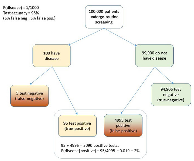
Cascells’ phrasing of his Harvard quiz was as follows: “If a test to detect a disease whose prevalence is 1 out of 1,000 has a false positive rate of 5 percent, what is the chance that a person found to have a positive result actually has the disease?”
Plugging in the numbers from the Cascells experiment (with the parameters Cascells provided shown below in bold and the correct answer in green):
- P(D) is the disease frequency = 0.001 [ 1 per 1000 in population ] therefore:
- P(not D) is 1 – P(D) = 0.999
- P(T | not D) = 5% = 0.05 [ false positive rate also 5%] therefore:
- P(T | D) = 95% = 0.95 [ i.e, the false negative rate is 5% ]
Substituting:
P(T) = .95 * .001 + .999 * .05 = 0.0509 ≈ 5.1% [ total probability of a positive test ]
P(D|T) = .95 * .001 / .0509 = .0019 ≈ 2% [ probability that patient has disease, given a positive test result ]
Voila.
I hope this seeing is believing illustration of Cascells’ experiment drives the point home for those still uneasy with equations. I used Cascells’ rates and a population of 100,000 to avoid dealing with fractional people:
Extra credit: how exactly does this apply to Covid, news junkies?
Edit 5/21/20. An astute reader called me on an inaccuracy in the diagram. I used an approximation, without identifying it. P = r1/r2 is a cheat for P = 1 – Exp(- r1/r2). The approximation is more intuitive, though technically wrong. It’s a good cheat, for P values less that 10%.
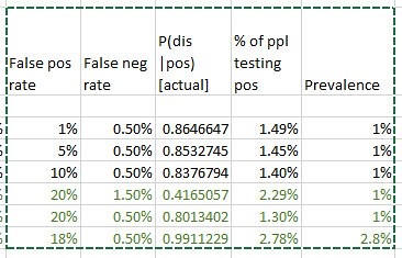
Note 5/22/20. In response to questions about how this sort of thinking bears on coronavirus testing -what test results say about prevalence – consider this. We really have one equation in 3 unknowns here: false positive rate, false negative rate, and prevalence in population. A quick Excel variations study using false positive rates from 1 to 20% and false neg rates from 1 to 3 percent, based on a quick web search for proposed sensitivity/specificity for the Covid tests is revealing. Taking the low side of the raw positive rates from the published data (1 – 3%) results in projected prevalence roughly equal to the raw positive rates. I.e., the false positives and false negatives happen to roughly wash out in this case. That also leaves P(d|t) in the range of a few percent.
Daniel Kahneman’s Bias Bias
Posted by Bill Storage in Probability and Risk on September 5, 2019
(3rd post on rational behavior of people too hastily judged irrational. See first and second.)
Daniel Kahneman has made great efforts to move psychology in the direction of science, particularly with his pleas for attention to replicability after research fraud around the priming effect came to light. Yet in Thinking Fast And Slow Kahneman still seems to draw some broad conclusions from a thin mantle of evidentiary icing upon a thick core of pre-formed theory. He concludes that people are bad intuitive Bayesians through flawed methodology and hypotheticals that set things up so that his psychology experiment subjects can’t win. Like many in the field of behavioral economics, he’s inclined to find bias and irrational behavior in situations better explained by the the subjects’ simply lacking complete information.
Like Richard Thaler and Dan Ariely, Kahneman sees bias as something deeply ingrained and hard-coded, programming that cannot be unlearned. He associates most innate bias with what he calls System 1, our intuitive, fast thinking selves. When called on to judge probability,” Kahneman says, “people actually judge something else and believe they have judged probability.” He agrees with Thaler, who finds “our ability to de-bias people is quite limited.”
But who is the “we” (“our” in that quote), and how is that “they” (Thaler, Ariely and Kahneman) are sufficiently unbiased to make this judgment? Are those born without the bias gene somehow drawn to the field of psychology; or through shear will can a few souls break free? If behavioral economists somehow clawed their way out of the pit of bias, can they not throw down a rope for the rest of us?
Take Kahneman’s example of the theater tickets. He compares two situations:
A. A woman has bought two $80 tickets to the theater. When she arrives at the theater, she opens her wallet and discovers that the tickets are missing. $80 tickets are still available at the box office. Will she buy two more tickets to see the play?
B. A woman goes to the theater, intending to buy two tickets that cost $80 each. She arrives at the theater, opens her wallet, and discovers to her dismay that the $160 with which she was going to make the purchase is missing. $80 tickets are still available at the box office. She has a credit card. Will she buy the tickets and just charge them?
Kahnemen says that the sunk-cost fallacy, a mental-accounting fallacy, and the framing effect account for the fact that many people view these two situations differently. Cases A and B are functionally equivalent, Kahneman says.
Really? Finding that $160 is missing from a wallet would cause most people to say, “darn, where did I misplace that money?”. Surely, no pickpocket removed the cash and stealthily returned the wallet to her purse. So the cash is unarguably a sunk cost in case A, but reasonable doubt exists in case B. She probably left the cash at home. As with philosophy, many problems in psychology boil down to semantics. And like the trolley problem variants, the artificiality of the problem statement is a key factor in the perceived irrationality of subjects’ responses.
By framing effect, Kahneman means that people’s choices are influenced by whether two options are presented with positive or negative connotations. Why is this bias? The subject has assumed that some level of information is embedded in the framer’s problem statement. If the psychologist judges that the subject has given this information too much weight, we might consider demystifying the framing effect by rebranding it the gullibility effect. But at that point it makes sense to question whether framing, in a broader sense, is at work in the thought problems. In presenting such problems and hypothetical situations to subjects, the framers imply a degree of credibility that is then used against those subjects by judging them irrational for accepting the conditions stipulated in the problem statement.
Bayesian philosophy is based on the idea of using a specific rule set for updating a “prior” (meaning prior belief – the degree of credence assigned to a claim or proposition) on the basis of new evidence. A Bayesian would interpret the framing effect, and related biases Kahneman calls anchoring and priming, as either a logic error in processing the new evidence or as a judgment error in the formation of an initial prior. The latter – how we establish initial priors – is probably the most enduring criticism of Bayesian reasoning. More on that issue later, but a Bayesian would say that Kayneman’s subjects need training in the use of uninformative priors and initial priors. Humans are shown to be very trainable in this matter, against the behavioral economists’ conclusion that we are hopelessly bound to innate bias.
One example Kahneman uses to show the framing effect presents different anchors to two separate test groups:
Group 1: Is the height of the tallest redwood more or less than 1200 feet? What is your best guess for the height of the tallest redwood?
Group 2: Is the height of the tallest redwood more or less than 120 feet? What is your best guess for the height of the tallest redwood?
Group 1’s average estimate was 844 feet, Group 2 gave 282 feet. The difference between the two anchors is 1080 feet. (1200 – 120). The difference in estimates by the two groups was 562 feet. Kahneman defines anchoring index as the ratio of the difference between mean estimates and difference in anchors. He uses this anchoring index to measure the robustness of the effect. He rules out the possibility that anchors are taken by subjects to be informative, saying that obviously random anchors can be just as effective, citing a 50% anchoring index when German judges rolled loaded dice (allowing only values of 3 or 9 to come up) before sentencing a shoplifter (hypothetical, of course). Kahneman reports that judges rolling a 3 gave 5-month sentences while those rolling a 9 assigned the shoplifter an 8-month sentence (index = 50%).
But the actual study (Englich, et. al.) cited by Kahneman has some curious aspects, besides the fact that it was very hypothetical. The judges found the fictional case briefs to be realistic, but they were not judging from the bench. They were working a thought problem. Englich’s Study 3 (the one Kahneman cites) shows the standard deviation in sentences was relatively large compared to the difference between sentences assigned by the two groups. More curious is a comparison of Englich’s Study 2 and the Study 3 Kahneman describes in Fast and Slow. Study 2 did not involve throwing dice to create an anchor. Its participants were only told that the prosecutor was demanding either a 3 or 9 month sentence, those terms not having originated in any judicial expertise. In Study 3, the difference between mean sentences from judges who received the two anchors was only two months (anchoring index = 33%).
Studies 2 and 3 therefore showed a 51% higher anchoring index for an explicitly random (clearly known to be random by participants) anchor than for an anchor understood by participants to be minimally informative. This suggests either that subjects regard pure chance as being more useful than potentially relevant information, or that something is wrong with the experiment, or that something is wrong with Kahnemnan’s inferences from evidence. I’ll suggest that the last two are at work, and that Kahneman fails to see that he is preferentially selecting confirming evidence over disconfirming evidence because he assumed his model of innate human bias was true before he examined the evidence. That implies a much older, more basic fallacy might be at work: begging the question, where an argument’s premise assumes the truth of the conclusion.
That fallacy is not an innate bias, however. It’s a rhetorical sin that goes way back. It is eminently curable. Aristotle wrote of it often and committed it slightly less often. The sciences quickly began to learn the antidote – sometimes called the scientific method – during the Enlightenment. Well, some quicker than others.
Let’s just fix the trolley
Posted by Bill Storage in Ethics, Philosophy on August 23, 2019
The classic formulation of the trolley-problem thought experiment goes something like this:
A runaway trolley hurtles toward five tied-up people on the main track. You see a lever that controls the switch. Pull it and the trolley switches to a side track, saving the five people, but will kill one person tied up on the side track. Your choices:
- Do nothing and let the trolley kill the five on the main track.
- Pull the lever, diverting the trolley onto the side track causing it to kill one person.
 At this point the Ethics 101 class debates the issue and dives down the rabbit hole of deontology, virtue ethics, and consequentialism. That’s probably what Philippa Foot, who created the problem, expected. At this point engineers probably figure that the ethicists mean cable-cars (below right), not trolleys (streetcars, left), since the cable cars run on steep hills and rely on a single, crude mechanical brake while trolleys tend to stick to flatlands. But I digress.
 Many trolley problem variants exist. The first twist usually thrust upon trolley-problem rookies was called “the fat man variant” back in the mid 1970s when it first appeared. I’m not sure what it’s called now.
The same trolley and five people, but you’re on a bridge over the tracks, and you can block it with a very heavy object. You see a very fat man next to you. Your only timely option is to push him over the bridge and onto the track, which will certainly kill him and will certainly save the five. To push or not to push.
Ethicists debate the moral distinction between the two versions, focusing on intentionality, double-effect reasoning etc. Here I leave the trolley problems in the competent hands of said ethicists.
But psychologists and behavioral economists do not. They appropriate the trolley problems as an apparatus for contrasting emotion-based and reason-based cognitive subsystems. At other times it becomes all about the framing effect, one of the countless cognitive biases afflicting the subset of souls having no psych education. This bias is cited as the reason most people fail to see the two trolley problems as morally equivalent.
The degree of epistemological presumptuousness displayed by the behavioral economist here is mind-boggling. (Baby, you don’t know my mind…, as an old Doc Watson song goes.) Just because it’s a thought experiment doesn’t mean it’s immune to the rules of good design of experiments. The fat-man variant is radically different from the original trolley formulation. It is radically different in what the cognizing subject imagines upon hearing/reading the problem statement. The first scenario is at least plausible in the real world, the second isn’t remotely.
First off, pulling the lever is about as binary as it gets: it’s either in position A or position B and any middle choice is excluded outright. One can perhaps imagine a real-world switch sticking in the middle, causing an electrical short, but that possibility is remote from the minds of all but reliability engineers, who, without cracking open MIL-HDBK-217, know the likelihood of that failure mode to be around one per 10 million operations.
Pushing someone, a very heavy someone, over the railing of the bridge is a complex action, introducing all sorts of uncertainty. Of course the bridge has a railing; you’ve never seen one that didn’t. There’s a good chance the fat man’s center of gravity is lower than the top of the railing because it was designed to keep people from toppling over it. That means you can’t merely push him over; you more have to lift him up to the point where his CG is higher than the top of railing. But he’s heavy, not particularly passive, and stronger than you are. You can’t just push him into the railing expecting it to break either. Bridge railings are robust. Experience has told you this for your entire life. You know it even if you know nothing of civil engineering and pedestrian bridge safety codes. And if the term center of gravity (CG) is foreign to you, by age six you have grounded intuitions on the concept, along with moment of inertia and fulcrums.
Assume you believe you can somehow overcome the railing obstacle. Trolleys weigh about 100,000 pounds. The problem statement said the trolley is hurtling toward five people. That sounds like 10 miles per hour at minimum. Your intuitive sense of momentum (mass times velocity) and your intuitive sense of what it takes to decelerate the hurtling mass (Newton’s 2nd law, f = ma) simply don’t line up with the devious psychologist’s claim that the heavy person’s death will save five lives. The experimenter’s saying it – even in a thought experiment – doesn’t make it so, or even make it plausible. Your rational subsystem, whether thinking fast or slow, screams out that the chance of success with this plan is tiny. So you’re very likely to needlessly kill your bridge mate, and then watch five victims get squashed all by yourself.
The test subjects’ failure to see moral equivalence between the two trolley problems speaks to their rationality, not their cognitive bias. They know an absurd hypothetical when they see one. What looks like humanity’s logical ineptitude to so many behavioral economists appears to the engineers as humanity’s cultivated pragmatism and an intuitive grasp of physics, factor-relevance evaluation, and probability.
There’s book smart, and then there’s street smart, or trolley-tracks smart, as it were.
My Trouble with Bayes
Posted by Bill Storage in Philosophy of Science, Probability and Risk, Uncategorized on January 21, 2016
 In past consulting work I’ve wrestled with subjective probability values derived from expert opinion. Subjective probability is an interpretation of probability based on a degree of belief (i.e., hypothetical willingness to bet on a position) as opposed a value derived from measured frequencies of occurrences (related posts: Belief in Probability, More Philosophy for Engineers). Subjective probability is of interest when failure data is sparse or nonexistent, as was the data on catastrophic loss of a space shuttle due to seal failure. Bayesianism is one form of inductive logic aimed at refining subjective beliefs based on Bayes Theorem and the idea of rational coherence of beliefs. A NASA handbook explains Bayesian inference as the process of obtaining a conclusion based on evidence, “Information about a hypothesis beyond the observable empirical data about that hypothesis is included in the inference.” Easier said than done, for reasons listed below.
Bayes Theorem itself is uncontroversial. It is a mathematical expression relating the probability of A given that B is true to the probability of B given that A is true and the individual probabilities of A and B:
P(A|B) = P(B|A) x P(A) / P(B)
If we’re trying to confirm a hypothesis (H) based on evidence (E), we can substitute H and E for A and B:
P(H|E) = P(E|H) x P(H) / P(E)
To be rationally coherent, you’re not allowed to believe the probability of heads to be .6 while believing the probability of tails to be .5; the sum of chances of all possible outcomes must sum to exactly one. Further, for Bayesians, the logical coherence just mentioned (i.e., avoidance of Dutch book arguments) must hold across time (synchronic coherence) such that once new evidence E on a hypothesis H is found, your believed probability for H given E should equal your prior conditional probability for H given E.
Plenty of good sources explain Bayesian epistemology and practice far better than I could do here. Bayesianism is controversial in science and engineering circles, for some good reasons. Bayesianism’s critics refer to it as a religion. This is unfair. Bayesianism is, however, like most religions, a belief system. My concern for this post is the problems with Bayesianism that I personally encounter in risk analyses. Adherents might rightly claim that problems I encounter with Bayes stem from poor implementation rather than from flaws in the underlying program. Good horse, bad jockey? Perhaps.
Problem 1. Subjectively objective
Bayesianism is an interesting mix of subjectivity and objectivity. It imposes no constraints on the subject of belief and very few constraints on the prior probability values. Hypothesis confirmation, for a Bayesian, is inherently quantitative, but initial hypotheses probabilities and the evaluation of evidence is purely subjective. For Bayesians, evidence E confirms or disconfirms hypothesis H only after we establish how probable H was in the first place. That is, we start with a prior probability for H. After the evidence, confirmation has occurred if the probability of H given E is higher than the prior probability of H, i.e., P(H|E) > P(H). Conversely, E disconfirms H when P(H|E) < P(H). These equations and their math leave business executives impressed with the rigor of objective calculation while directing their attention away from the subjectivity of both the hypothesis and its initial prior.
2. Rational formulation of the prior
Problem 2 follows from the above. Paranoid, crackpot hypotheses can still maintain perfect probabilistic coherence. Excluding crackpots, rational thinkers – more accurately, those with whom we agree – still may have an extremely difficult time distilling their beliefs, observations and observed facts of the world into a prior.
3. Conditionalization and old evidence
This is on everyone’s short list of problems with Bayes. In the simplest interpretation of Bayes, old evidence has zero confirming power. If evidence E was on the books long ago and it suddenly comes to light that H entails E, no change in the value of H follows. This seems odd – to most outsiders anyway. This problem gives rise to the game where we are expected to pretend we never knew about E and then judge how surprising (confirming) E would have been to H had we not know about it. As with the general matter of maintaining logical coherence required for the Bayesian program, it is extremely difficult to detach your knowledge of E from the rest of your knowing about the world. In engineering problem solving, discovering that H implies E is very common.
4. Equating increased probability with hypothesis confirmation.
My having once met Hillary Clinton arguably increases the probability that I may someday be her running mate; but few would agree that it is confirming evidence that I will do so. See Hempel’s raven paradox.
5. Stubborn stains in the priors
Bayesians, often citing success in the business of establishing and adjusting insurance premiums, report that the initial subjectivity (discussed in 1, above) fades away as evidence accumulates. They call this washing-out of priors. The frequentist might respond that with sufficient evidence your belief becomes irrelevant. With historical data (i.e., abundant evidence) they can calculate P of an unwanted event in a frequentist way: P = 1-e to the power -RT, roughly, P=RT for small products of exposure time T and failure rate R (exponential distribution). When our ability to find new evidence is limited, i.e., for modeling unprecedented failures, the prior does not get washed out.
6. The catch-all hypothesis
The denominator of Bayes Theorem, P(E), in practice, must be calculated as the sum of the probability of the evidence given the hypothesis plus the probability of the evidence given not the hypothesis:
P(E) = [P(E|H) x p(H)] + [P(E|~H) x P(~H)]
But ~H (“not H”) is not itself a valid hypothesis. It is a family of hypotheses likely containing what Donald Rumsfeld famously called unknown unknowns. Thus calculating the denominator P(E) forces you to pretend you’ve considered all contributors to ~H. So Bayesians can be lured into a state of false choice. The famous example of such a false choice in the history of science is Newton’s particle theory of light vs. Huygens’ wave theory of light. Hint: they are both wrong.
7. Deference to the loudmouth
This problem is related to no. 1 above, but has a much more corporate, organizational component. It can’t be blamed on Bayesianism but nevertheless plagues Bayesian implementations within teams. In the group formulation of any subjective probability, normal corporate dynamics govern the outcome. The most senior or deepest-voiced actor in the room drives all assignments of subjective probability. Social influence rules and the wisdom of the crowd succumbs to a consensus building exercise, precisely where consensus is unwanted. Seidenfeld, Kadane and Schervish begin “On the Shared Preferences of Two Bayesian Decision Makers” with the scholarly observation that an outstanding challenge for Bayesian decision theory is to extend its norms of rationality from individuals to groups. Their paper might have been illustrated with the famous photo of the exploding Challenger space shuttle. Bayesianism’s tolerance of subjective probabilities combined with organizational dynamics and the shyness of engineers can be a recipe for disaster of the Challenger sort.
All opinions welcome.
A New Era of Risk Management?
Posted by Bill Storage in Probability and Risk, Risk Management on February 9, 2014
The quality of risk management has mostly fallen for the past few decades. There are signs of change for the better.
Risk management is a broad field; many kinds of risk must be managed. Risk is usually defined in terms of probability and cost of a potential loss. Risk management, then, is the identification, assessment and prioritization of risks and the application of resources to reduce the probability and/or cost of the loss.
The earliest and most accessible example of risk management is insurance, first documented in about 1770 BC in the Code of Hammurabi (e.g., rules 23, 24, and 48). The Code addresses both risk mitigation, through threats and penalties, and minimizing loss to victims, through risk pooling and insurance payouts.
 Insurance was the first example of risk management getting serious about risk assessment. Both the frequentist and quantified subjective risk measurement approaches (see recent posts on belief in probability) emerged from actuarial science developed by the insurance industry.
Risk assessment, through its close relatives, decision analysis and operations research, got another boost from World War II. Big names like Alan Turing, John Von Neumann, Ian Fleming (later James Bond author) and teams at MIT, Columbia University and Bletchley Park put quantitative risk analyses of several flavors on the map.
Today, “risk management” applies to security guard services, portfolio management, terrorism and more. Oddly, much of what is called risk management involves no risk assessment at all, and is therefore inconsistent with the above definition of risk management, paraphrased from Wikipedia.
Most risk assessment involves quantification of some sort. Actuarial science and the probabilistic risk analyses used in aircraft design are probably the “hardest” of the hard risk measurement approaches, Here, “hard” means the numbers used in the analyses come from measurements of real world values like auto accidents, lightning strikes, cancer rates, and the historical failure rates of computer chips, valves and motors. “Softer” analyses, still mathematically rigorous, involve quantified subjective judgments in tools like Monte Carlo analyses and Bayesian belief networks. As the code breakers and submarine hunters of WWII found, trained experts using calibrated expert opinions can surprise everyone, even themselves.
A much softer, yet still quantified (barely), approach to risk management using expert opinion is the risk matrix familiar to most people: on a scale of 1 to 4, rate the following risks…, etc. It’s been shown to be truly worse than useless in many cases, for a variety of reasons by many researchers. Yet it remains the core of risk analysis in many areas of business and government, across many types of risk (reputation, credit, project, financial and safety). Finally, some of what is called risk management involves no quantification, ordering, or classifying. Call it expert intuition or qualitative audit.
These soft categories of risk management most arouse the ire of independent and small-firm risk analysts. Common criticisms by these analysts include:
1. “Risk management” has become jargonized and often involves no real risk analysis.
2. Quantification of risk in some spheres is plagued by garbage-in-garbage-out. Frequency-based models are taken as gospel, and believed merely because they look scientific (e.g., Fukushima).
3. Quantified/frequentist risk analyses are not used in cases where historical data and a sound basis for them actually exists (e.g., pharmaceutical manufacture).
4. Big consultancies used their existing relationships to sell unsound (fluff) risk methods, squeezing out analysts with sound methods (accused of Arthur Anderson, McKinsey, Bain, KPMG).
5. Quantitative risk analyses of subjective type commonly don’t involve training or calibration of those giving expert opinions, thereby resulting in incoherent (in the Bayesian sense) belief systems.
6. Groupthink and bad management override rational input into risk assessment (subprime mortgage, space shuttle Challenger).
7. Risk management is equated with regulatory compliance (banking operations, hospital medicine, pharmaceuticals, side-effect of Sarbanes-Oxley).
8. Some professionals refuse to accept any formal approach to risk management (medical practitioners and hospitals).
While these criticisms may involve some degree of sour grapes, they have considerable merit in my view, and partially explain the decline in quality of risk management. I’ve worked in risk analysis involving uranium processing, nuclear weapons handling, commercial and military aviation, pharmaceutical manufacture, closed-circuit scuba design, and mountaineering. If the above complaints are valid in these circles – and they are – it’s easy to believe they plague areas where softer risk methods reign.
Several books and scores of papers specifically address the problems of simple risk-score matrices, often dressed up in fancy clothes to look rigorous. The approach has been shown to have dangerous flaws by many analysts and scholars, e.g., Tony Cox, Sam Savage, Douglas Hubbard, and Laura-Diana Radu. Cox shows examples where risk matrices assign higher qualitative ratings to quantitatively smaller risks. He shows that risks with negatively correlated frequencies and severities can result in risk-matrix decisions that are worse than random decisions. Also, such methods are obviously very prone to range compression errors. Most interestingly, in my experience, the stratification (highly likely, somewhat likely, moderately likely, etc.) inherent in risk matrices assume common interpretation of terms across a group. Many tests (e.g., Kahneman & Tversky and Budescu, Broomell, Por) show that large differences in the way people understand such phrases dramatically affect their judgments of risk. Thus risk matrices create the illusion of communication and agreement where neither are present.
Nevertheless, the risk matrix has been institutionalized. It is embraced by government (MIL-STD-882), standards bodies (ISO 31000), and professional societies (Project Management Institute (PMI), ISACA/COBIT). Hubbard’s opponents argue that if risk matrices are so bad, why do so many people use them – an odd argument, to say the least. ISO 31000, in my view, isn’t a complete write-off. In places, it rationally addresses risk as something that can be managed through reduction of likelihood, reduction of consequences, risk sharing, and risk transfer. But elsewhere it redefines risk as mere uncertainty, thereby reintroducing the positive/negative risk mess created by economist Frank Knight a century ago. Worse, from my perspective, like the guidelines of PMI and ISACA, it gives credence to structure in the guise of knowledge and to process posing as strategy. In short, it sets up a lot of wickets which, once navigated, give a sense that risk has been managed when in fact it may have been merely discussed.
A small benefit of the subprime mortgage meltdown of 2008 was that it became obvious that the financial risk management revolution of the 1990s was a farce, exposing a need for deep structural changes. I don’t follow financial risk analysis closely enough to know whether that’s happened. But the negative example made public by the housing collapse has created enough anxiety in other disciplines to cause some welcome reappraisals.
There is surprising and welcome activity in nuclear energy. Several organizations involved in nuclear power generation have acknowledged that we’ve lost competency in this area, and have recently identified paths to address the challenges. The Nuclear Energy Institute recently noted that while Fukushima is seen as evidence that probabilistic risk analysis (PRA) doesn’t work, if Japan had actually embraced PRA, the high risk of tsunami-induced disaster would have been immediately apparent. Late last year the Nuclear Energy Institute submitted two drafts to the U.S. Nuclear Regulatory Commission addressing lost ground in PRA and identifying a substantive path forward: Reclaiming the Promise of Risk-Informed Decision-Making and Restoring Risk-Informed Regulation. These documents acknowledge that the promise of PRA has been stunted by distrust of the method, focus on compliance instead of science, external audits by unqualified teams, and the above-mentioned Fukushima fallacy.
Likewise, the FDA, often criticized for over-regulating and over-reach – confusing efficacy with safety – has shown improvement in recent years. It has revised its decades-old process validation guidance to focus more on verification, scientific evidence and risk analysis tools rather than validation and documentation. The FDA’s ICH Q9 (Quality Risk Management) guidelines discuss risk, risk analysis and risk management in terms familiar to practitioners of “hard” risk analysis, even covering fault tree analysis (the “hardest” form of PRA) in some detail. The ASTM E2500 standard moves these concepts further forward. Similarly, the FDA’s recent guidelines on mobile health devices seem to accept that the FDA’s reach should not exceed its grasp in the domain of smart phones loaded with health apps. Reading between the lines, I take it that after years of fostering the notion that risk management equals regulatory compliance, the FDA realized that it must push drug safety far down into the ranks of the drug makers in the same way the FAA did with aircraft makers (with obvious success) in the late 1960s. Fostering a culture of safety rather than one of compliance distributes the work of providing safety and reduces the need for regulators to anticipate every possible failure of every step of every process in every drug firm.
This is real progress. There may yet be hope for financial risk management.
Belief in Probability – Part 2
Posted by Bill Storage in Probability and Risk, Systems Engineering on December 19, 2013
 Last time I started with my friend Willie’s bold claim that he doesn’t believe in probability; then I gave a short history of probability. I observed that defining probability is a controversial matter, split between objective and subjective interpretations. About the only thing these interpretations agree on is that probability values range from zero to one, where P = 1 means certainty. When you learn probability and statistics in school, you are getting the frequentist interpretation, which is considered objective. Frequentism relies on directly equating observed frequencies with probabilities. In this model, the probability of an event exactly equals the limit of the relative frequency of that outcome in an infinitely large number of trials.
The problem with this interpretation in practice – in medicine, engineering, and gambling machines – isn’t merely the impossibility of an infinite number of trials. A few million trials might be enough. Running trials works for dice but not for earthquakes and space shuttles. It also has problems with things like cancer, where plenty of frequency data exists. Frequentism requires placing an individual specimen into a relevant population or reference class. Doing this is easy for dice, harder for humans. A study says that as a white males of my age I face a 7% probability of having a stroke in the next 10 years. That’s based on my membership in the reference class of white males. If I restrict that set to white men who don’t smoke, it drops to 4%. If I account for good systolic blood pressure, no family history of atrial fibrillation or ventricular hypertrophy, it drops another percent or so.
Ultimately, if I limit my population to a set of one (just me) and apply the belief that every effect has a cause (i.e., some real-world chunk of blockage causes an artery to rupture), you can conclude that my probability of having a stroke can only be one of two values – zero or one.
Frequentism, as seen by its opponents, too closely ties probabilities to observed frequencies. They note that the limit-of-relative-frequency concept relies on induction, which might mean it’s not so objective after all. Further, those frequencies are unknowable in many real-world cases. Still further, finding an individual’s correct reference class is messy, possibly downright subjective. Finally, no frequency data exists for earthquakes that haven’t happened yet. All that seems to do some real damage to frequentism’s utility score.
The subjective interpretations of probability propose fixes to some of frequentism’s problems. The most common subjective interpretation is Bayesianism, which itself comes in several flavors. All subjective interpretations see probability as a degree of belief in a specific outcome, as held by a rational person. Think of it as a fair bet with odds. The odds you’re willing to accept for a bet on your race horse exactly equals your degree of belief in that horse’s ability to win. If your filly were in the same race an infinite number of times, you’d expect to break even, based on those odds, whether you bet on her or against her.
Subjective interpretations rely on logical coherence and belief. The core of Bayesianism, for example, is that beliefs must 1) originate with a numerical probability estimate, 2) adhere to the rules of probability calculation, and 3) follow an exact rule for updating belief estimates based on new evidence. The second rule deals with the common core of probability math used in all interpretations. These include things like how to add and multiply probabilities and Bayes theorem, not to be confused with Bayesianism, the belief system. Bayes theorem is an uncontroversial equation relating the probability of A given B to the probability of A and the probability of B. The third rule of Bayesianism is similarly computational, addressing how belief is updated after new evidence. The details aren’t needed here. Note that while Bayesianism is generally considered subjective, it is still computationally exacting.
The obvious problem with all subjective interpretations, particularly as applied to engineering problems, is that they rely, at least initially, on expert opinion. Life and death rides on the choice of experts and the value of their opinions. As Richard Feynman noted in his minority report on the Challenger, official rank plays too large a part in the choice of experts, and the higher (and less technical) the rank, the more optimistic the probability estimates.
The engineering risk analysis technique most consistent with the frequentist (objective) interpretation of probability is fault tree analysis. Other risk analysis techniques, some embodied in mature software products, are based on Bayesian (subjective) philosophy.
When Willie said he didn’t believe in probability, he may have meant several things. I’ll try to track him down and ask him, but I doubt the incident stuck in his mind as it did mine. If he meant that he doesn’t believe that probability was useful in system design, he had a rational belief; but I disagree with it. I doubt he meant that though.
Willie may have been leaning toward the ties between probability and redundancy in system design. Probability is the calculus by which redundancy is allocated to redundant systems. Willie may think that redundancy doesn’t yield the expected increase in safety because having more equipment means more things than can fail. This argument fails to face that, ideally speaking, a redundant path does double the chance having a component failure, but squares the probability of system failure. That’s a good thing, since squaring a number less than one makes it smaller. In other words, the benefit in reducing the chance of system failure vastly exceeds the deficit of having more components to repair. If that was his point, I disagree in principle, but accept that redundancy is no excuse for lack of component design excellence.
He may also think system designers can be overly confident of the exponential increase in modeled probability of system reliability that stems from redundancy. That increase in reliability is only valid if the redundancy creates no common mode failures and no latent (undetected for unknown time intervals) failures of redundant paths that aren’t currently operating. If that’s his point, then we agree completely. This is an area where pairing the experience and design expertise of someone like Willie with rigorous risk analysis using fault trees yields great systems.
Unlike Willie, Challenger-era NASA gave no official statement on its belief in probability. Feynman’s report points to NASA’s use of numeric probabilities for specific component failure modes. The Rogers Commission report says that NASA management talked about degrees of probability. From this we might guess that NASA believed in probability and its use in measuring risk. On the other hand, the Rogers Commission report also gives examples of NASA’s disbelief in probability’s usefulness. For example, the report’s Technical Management section states that, “NASA has rejected the use of probability on the basis that such techniques are insufficient to assure that adequate safety margins can be applied to protect the lives of the crew.”
Regardless of what NASA’s beliefs about porbability, it’s clear that NASA didn’t use fault tree analysis for the space shuttle program prior to the Challenger disaster. Nor did it use Bayesian inference methods, any hybrid probability model, or any consideration of probability beyond opinions about failures of critical items. Feynman was livid about this. A Bayesian (subjective, but computational) approach would have at least forced NASA to make it subjective judgments explicit and would have produced a rational model of its judgments. Post-Challenger Bayesian analyses, including one by NASA, varied widely, but all indicated unacceptable risk. NASA has since adopted risk management approaches more consistent with those used in commercial and military aircraft design.
An obvious question arises when you think about using a frequentist model on nearly one-of-a-kind vehicles. How accurate can any frequency data be for something as infrequent as a shuttle flight? Accurate enough, in my view. If you see the shuttle as monolithic and indivisible, the data is too sparse; but not if you view it as a system of components, most of which, like o-ring seals, have close analogs in common use, with known failure rates.
The FAA mandated probabilistic risk analyses of the frequentist variety (effectively mandating fault trees) in 1968. Since then flying has become safe, by any measure. In no other endeavor has mankind made such an inherently dangerous activity so safe. Aviation safety progressed through many innovations, redundant systems being high on the list. Probability is the means by which you allocate redundancy. You can’t get great aircraft systems without designers like Willie. Nor can you get them without probability. Believe it or not.
Belief in Probability – Part 1
Posted by Bill Storage in Aerospace, Probability and Risk, Risk Management, Systems Engineering on December 18, 2013
Years ago in a meeting on design of a complex, redundant system for a commercial jet, I referred to probabilities of various component failures. In front of this group of seasoned engineers, a highly respected, senior member of the team interjected, “I don’t believe in probability.” His proclamation stopped me cold. My first thought was what kind a backward brute would say something like that, especially in the context of aircraft design. But Willie was no brute. In fact he is a legend in electro-hydro-mechanical system design circles; and he deserves that status. For decades, millions of fearless fliers have touched down on the runway, unaware that Willie’s expertise played a large part in their safe arrival. So what can we make of Willie’s stated disbelief in probability?

Friends and I have been discussing risk science a lot lately – diverse aspects of it including the Challenger disaster, pharmaceutical manufacture in China, and black swans in financial markets. I want to write a few posts on risk science, as a personal log, and for whomever else might be interested. Risk science relies on several different understandings of risk, which in turn rely on the concept of probability. So before getting to risk, I’m going to jot down some thoughts on probability. These thoughts involve no computation or equations, but they do shed some light on Willie’s mindset. First a bit of background.
Oddly, the meaning of the word probability involves philosophy much more than it does math, so Willie’s use of belief might be justified. People mean very different things when they say probability. The chance of rolling a 7 is conceptually very different from the chance of an earthquake in Missouri this year. Probability is hard to define accurately. A look at its history shows why.
Mathematical theories of probability only first appeared in the late 17th century. This is puzzling, since gambling had existed for thousands of years. Gambling was enough of a problem in the ancient world that the Egyptian pharaohs, Roman emperors and Achaemenid satraps outlawed it. Such legislation had little effect on the urge to deal the cards or roll the dice. Enforcement was sporadic and halfhearted. Yet gamblers failed to develop probability theories. Historian Ian Hacking (The Emergence of Probability) observes, “Someone with only the most modest knowledge of probability mathematics could have won himself the whole of Gaul in a week.”
Why so much interest with so little understanding? In European and middle eastern history, it seems that neither Platonism (determinism derived from ideal forms) nor the Judeo/Christian/Islamic traditions (determinism through God’s will) had much sympathy for knowledge of chance. Chance was something to which knowledge could not apply. Chance meant uncertainty, and uncertainty was the absence of knowledge. Knowledge of chance didn’t seem to make sense. Plus, chance was the tool of immoral and dishonest gamblers.
The term probability is tied to the modern understanding of evidence. In medieval times, and well into the renaissance, probability literally referred to the level of authority – typically tied to the nobility – of a witness in a court case. A probable opinion was one given by a reputable witness. So a testimony could be highly probable but very incorrect, even false.
Through empiricism, central to the scientific method, the notion of diagnosis (inference of a condition from key indicators) emerged in the 17th century. Diagnosis allowed nature to be the reputable authority, rather than a person of status. For example, the symptom of skin spots could testify, with various degrees of probability, that measles had caused it. This goes back to the notion of induction and inference from the best explanation of evidence, which I discussed in past posts. Pascal, Fermat and Huygens brought probability into the respectable world of science.
But outside of science, probability and statistics still remained second class citizens right up to the 20th century. You used these tools when you didn’t have an exact set of accurate facts. Recognition of the predictive value of probability and statistics finally emerged when governments realized that death records had uses beyond preserving history, and when insurance companies figured out how to price premiums competitively.
Also around the turn of the 20th century, it became clear that in many realms – thermodynamics and quantum mechanics for example – probability would take center stage against determinism. Scientists began to see that some – perhaps most – aspects of reality were fundamentally probabilistic in nature, not deterministic. This was a tough pill for many to swallow, even Albert Einstein. Einstein famously argued with Niels Bohr, saying, “God does not play dice.” Einstein believed that some hidden variable would eventually emerge to explain why one of two identical atoms would decay while the other did not. A century later, Bohr is still winning that argument.
What we mean when we say probability today may seem uncontroversial – until you stake lives on it. Then it gets weird, and definitions become important. Defining probability is a wickedly contentious matter, because wildly conflicting conceptions of probability exist. They can be roughly divided into the objective and subjective interpretations. In the next post I’ll focus on the frequentist interpretation, which is objective, and the subjectivist interpretations as a group. I’ll look at the impact of accepting – or believing in – each of these on the design of things like airliners and space shuttles from the perspectives of Willie, Richard Feynman, and NASA. Then I’ll defend my own views on when and where to hold various beliefs about probability.
Intuitive Probabilities
Posted by Bill Storage in Probability and Risk on October 1, 2013
 Meet Vic. Vic enjoys a form of music that features heavily distorted guitars, slow growling vocals, atonality, frequent tempo changes, and what is called “blast beat” drumming in the music business. His favorite death metal bands are Slayer, Leviticus, Dark Tranquility, Arch Enemy, Behemoth, Kreator, Venom, and Necrophagist.
Vic has strong views on theology and cosmology. Which is more likely?
- Vic is a Christian
- Vic is a Satanist
I’ve taught courses on probabilistic risk analysis over the years, and have found that very intelligent engineers, much more experienced than I, often find probability extremely unintuitive. Especially when very large (or very small) numbers are involved. Other aspects of probability and statistics are unintuitive for other interesting reasons. More on those later.
The matter of Vic’s belief system involves several possible biases and unintuitive aspects of statistics. While pondering the issue of Vic’s beliefs, you can enjoy Slayer’s Raining Blood. Then check out my take on judging Vic’s beliefs below the embedded YouTube video – which, by the way, demonstrates all of the attributes of death metal listed above.
.
Vic is almost certainly a Christian. Any other conclusion would involve the so-called base-rate fallacy, where the secondary, specific facts (affinity for death metal) somehow obscure the primary, base-rate relative frequency of Christians versus Satanists. The Vatican claims over one billion Catholics, and most US Christians are not Catholic. Even with papal exaggeration, we can guess that there are well over a billion Christians on earth. I know hundreds if not thousands of them. I don’t know any Satanists personally, and don’t know of any public figures who are (there is conflicting evidence on Marilyn Manson). A quick Google search suggests a range of numbers of Satanists in the world, the largest of which is under 100,000. Further, I don’t ever remember seeing a single Satanist meeting facility, even in San Francisco. A web search also reveals a good number of conspicuously Christian death metal bands, including Leviticus, named above. Without getting into the details of Bayes Theorem, it is probably obvious that the relative frequencies of Christians against Satanists governs the outcome. And judging Vic by his appearance is likely very unreliable.

South Park Community Presbyterian Church
Fairplay, Colorado
