Archive for category Probability and Risk
“He Tied His Lace” – Rum, Grenades and Bayesian Reasoning in Peaky Blinders
Posted by Bill Storage in Probability and Risk on August 4, 2025
“He tied his lace.” Spoken by a jittery subordinate halfway through a confrontation, the line turns a scene in Peaky Blinders from stylized gangster drama into a live demonstration of Bayesian belief update. The scene is a tightly written jewel of deadpan absurdity.
(The video clip and a script excerpt from Season 2, Episode 6 appears at the bottom of this article – rough language. “Peaky blinders,” for what its worth, refers to young brits in blindingly dapper duds and peaked caps in the 1920s.)
The setup: Alfie Solomons has temporarily switched his alliance from Tommy Shelby to Darby Sabini, a rival Italian gangster, in exchange for his bookies being allowed at the Epsom Races. Alfie then betrayed Tommy by setting up Tommy’s brother Arthur and having him arrested for murder. But Sabini broke his promise to Alfie, causing Alfie to seek a new deal with Tommy. Now Tommy offers 20% of his bookie business. Alfie wants 100%. In the ensuing disagreement, Alfie’s man Ollie threatens to shoot Tommy unless Alfie’s terms are met.
Tommy then offers up a preposterous threat. He claims to have planted a grenade and wired it to explode if he doesn’t walk out the door by 7pm. The lynchpin of this claim? That he bent down to tie his shoe on the way in, thereby concealing his planting the grenade among Alfie’s highly flammable bootleg rum kegs. Ollie falls apart when, during the negotiations, he recalls seeing Tommy tie his shoe on the way in. “He tied his lace,” he mutters frantically.
In another setting, this might be just a throwaway line. But here, it’s the final evidence given in a series of Bayesian belief updates – an ambiguous detail that forces a final shift in belief. This is classic Bayesian decision theory with sequential Bayesian inference, dynamic belief updates, and cost asymmetry. Agents updates their subjective probability (posterior) based on new evidence and choose an action to maximize expected utility.
By the end of the negotiation, Alfie’s offering a compromise. What changes is not the balance of lethality or legality, but this sequence of increasingly credible signals that Tommy might just carry through on the threat in response to Alfie’s demands.
As evidence accumulates – some verbal, some circumstantial – Alfie revises his belief, lowers his demands, and eventually accepts a deal that reflects the posterior probability that Tommy is telling the truth. It’s Bayesian updating with combustible rum, thick Cockney accents, and death threats delivered with stony precision.
Bayesian belief updating involves (see also *):
- Prior belief (P(H)): Initial credence in a hypothesis (e.g., “Tommy is bluffing”).
- Evidence (E): New information (e.g., a credible threat of violence, or a revealed inconsistency).
- Likelihood (P(E|H)): How likely the evidence is if the hypothesis is true.
- Posterior belief (P(H|E)): Updated belief in the hypothesis given the evidence.
In Peaky Blinders, the characters have beliefs about each other’s natures, e.g., ruthless, crazy, bluffing.
The Exchange as Bayesian Negotiation
Initial Offer – 20% (Tommy)
This reflects Tommy’s belief that Alfie will find the offer worthwhile given legal backing and mutual benefits (safe rum shipping). He assumes Alfie is rational and profit-oriented.
Alfie’s Counter – 100%
Alfie reveals a much higher demand with a threat attached (Ollie + gun). He’s signaling that he thinks Tommy has little to no leverage – a strong prior that Tommy is bluffing or weak.
Tommy’s Threat – Grenade
Tommy introduces new evidence: a possible suicide mission, planted grenade, anarchist partner. Alfie must now update his beliefs:
- What is the probability Tommy is bluffing?
- What’s the chance the grenade exists and is armed?
Ollie’s Confirmation – “He tied his lace…”
This is independent corroborating evidence – evidence of something anyway. Alfie now receives a report that raises the likelihood Tommy’s story is true (P(E|¬H) drops, P(E|H) rises). So Alfie updates his belief in Tommy’s credibility, lowering his confidence that he can push for 100%.
The offer history, which controls their priors and posteriors:
- Alfie lowers from 100% → 65% (“I’ll bet 100 to 1”)
- Tommy rejects
- Alfie considers Tommy’s past form (“he blew up his own pub”)
This shifts the prior. Now P(Tommy is reckless and serious) is higher. - Alfie: 65% → 45%
- Tommy: Counters with 30%
- Tommy adds detail: WWI tunneling expertise, same grenade kit, he blew up a mine
- Alfie checks for inconsistency (“I heard they all got buried”)
Potential Bayesian disconfirmation. Is Tommy lying? - Tommy: “Three of us dug ourselves out” → resolves inconsistency
The model regains internal coherence. Alfie’s posterior belief in the truth of the grenade story rises again. - Final offer: 35%
They settle, each having adjusted credence in the other’s threat profile and willingness to follow through.
Analysis
Beliefs are not static. Each new statement, action, or contradiction causes belief shifts. Updates are directional, not precise. No character says “I now assign 65% chance…” but, since they are rational actors, their offers directly encode these shifts in valuation. We see behaviorally expressed priors and posteriors. Alfie’s movement from 100 to 65 to 45 to 35% is not arbitrary. It reflects updates in how much control he believes he has.
Credibility is a Bayesian variable. Tommy’s past (blowing up his own pub) is treated as evidence relevant to present behavior. Social proof is given by Ollie. Ollie panics on recalling that Tommy tied his shoe. Alfie chastises Ollie for being a child in a man’s world and sends him out. But Alfie has already processed this Bayesian evidence for the grenade threat, and Tommy knows it. The 7:00 deadline adds urgency and tension to the scene. Crucially, from a Bayesian perspective, it limits the number of possible belief revisions, a typical constraint for bounded rationality.
As an initial setup, let:
- T = Tommy has rigged a grenade
- ¬T = Tommy is bluffing
- P(T) = Alfie’s prior that Tommy is serious
Let’s say initially:
P(T) = 0.15, so P(¬T) = 0.85
Alfie starts with a strong prior that Tommy’s bluffing. Most people wouldn’t blow themselves up. Tommy’s a businessman, not a suicide bomber. Alfie has armed men and controls the room.
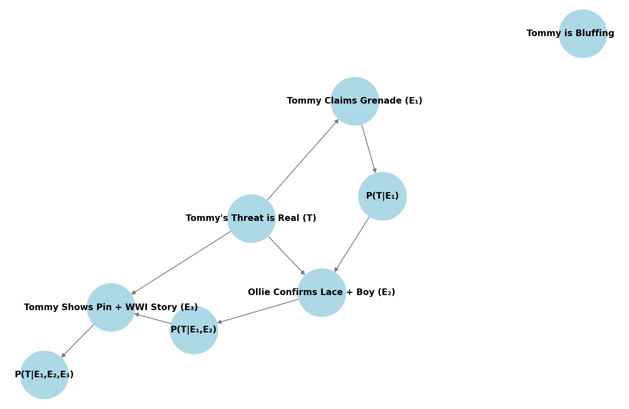
Sequence of Evidence and Belief Updates
Evidence 1: Tommy’s grenade threat
E₁ = Tommy says he planted a grenade and has an assistant with a tripwire
We assign:
- P(E₁|T) = 1 (he would say so if it’s real)
- P(E₁|¬T) = 0.7 (he might bluff this anyway)
Using Bayes’ Theorem:
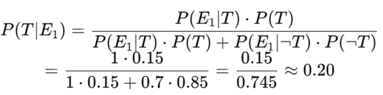
So now Alfie gives a 20% chance Tommy is telling the truth. Behavioral result: Alfie lowers the offer from 100% → 65%.
Evidence 2: Ollie confirms the lace-tying + nervousness
E₂ = Ollie confirms Tommy bent down and there’s a boy at the door
This is independent evidence supporting T.
- P(E₂|T) = 0.9 (if it’s true, this would happen)
- P(E₂|¬T) = 0.3 (could be coincidence)
Update:
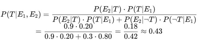
So Alfie now gives 43% probability that the grenade is real. Behavioral result: Offer drops to 45%.
Evidence 3: Tommy shows grenade pin + WWI tunneler claim
E₃ = Tommy drops the pin and references real tunneling experience
- P(E₃|T) = 0.95 (he’d be prepared and have a story)
- P(E₃|¬T) = 0.5 (he might fake this, but riskier)
Update:
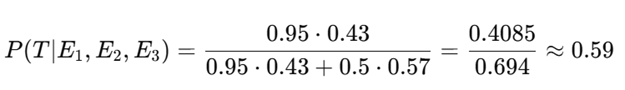
Now Alfie believes there’s nearly a 60% chance Tommy is serious. Behavioral result: Offer rises slightly to 35%, the final deal.
Simplified Utility Function
Assume Alfie’s utility is:
U(percent) = percent ⋅ V−C ⋅ P(T)
Where:
- V = Value of Tommy’s export business (let’s say 100)
- C = Cost of being blown up (e.g., 1000)
- P(T) = Updated belief Tommy is serious
So for 65%, with P(T) = 0.43:
U = 65 – 1000 ⋅ 0.43 = 65 – 430 = −365
But for 35%, with P(T) = 0.59:
U = 35 – 1000 ⋅ 0.59 = 35 – 590 = −555
Here we should note that Alfie’s utility function is not particularly sensitive to the numerical values of V and C; using C = 10,000 or 500 doesn’t change the relative outcomes much. So, why does Alfie accept the lower utility? Because risk of total loss is also a factor. If the grenade is real, pushing further ends in death and no gain. Alfie’s risk appetite is negatively skewed.
At the start of the negotiation, Alfie behaves like someone with low risk aversion by demanding 100%, assuming dominance, and later believing Tommy is bluffing. His prior is reflect extreme confidence and control. But as the conversation progresses, the downside risk becomes enormous: death, loss of business, and, likely worse, public humiliation.
The evidence increasingly supports the worst-case scenario. There’s no compensating upside for holding firm, no added reward for risking everything to get 65% instead of 35%.
This flips Alfie’s profile. He develops a sharp negative skew in risk appetite, especially under time pressure and mounting evidence. Even though 35% yields a worse expected utility than 65%, it avoids the long tail – catastrophic loss.
***
[Tommy is seated in Alfie’s office]
Alfie (to Tommy): That’ll probably be for you, won’t it?
Tommy: Hello? Arthur. You’re out.
Alfie: Right, so that’ll be your side of the street swept up, won’t it? Where’s mine? What you got for me?
Tommy: Signed by the Minister of the Empire himself. Yeah? So it is.
Tommy: This means that you can put your rum in our shipments, and no one at Poplar Docks will lift a canvas.
Alfie: You know what? I’m not even going to have my lawyer look at that.
Tommy: I know, it’s all legal.
Alfie: You know what, mate, I trust you. That’s that. Done. So, whisky… There is, uh, one thing, though, that we do need to discuss.
Tommy: What would that be?
Alfie: It says here, “20% “paid to me of your export business.”
Tommy: As we agreed on the telephone…
Alfie: No, no, no, no, no. See, I’ve had my lawyer draw this up for us, just in case. It says that, here, that 100% of your business goes to me.
Tommy: I see.
Alfie: It’s there.
Tommy: Right.
Alfie: Don’t worry about it, right, because it’s totally legal binding. All you have to do is sign the document and transfer the whole lot over to me.
Tommy: Sign just here, is it?
Alfie: Yeah.
Tommy: I see. That’s funny. That is.
Alfie: What?
Tommy: No, that’s funny. I’ll give you 100% of my business.
Alfie: Yeah.
Tommy: Why?
[Ollie appears and aims a revolver at Tommy]
Alfie: Ollie, no. No, no, no. Put that down. He understands, he understands. He’s a big boy, he knows the road. Now, look, it’s just non-fucking-negotiable. That’s all you need to know. So all you have to do is sign the fucking contract. Right there.
Tommy: just sign here?
Alfie: With your pen.
Tommy: I understand.
Alfie: Good. Get on with it.
Tommy: Well, I have an associate waiting for me at the door. I know that he looks like a choir boy, but he is actually an anarchist from Kentish Town.
Alfie: Tommy… I’m going to fucking shoot you. All right?
Tommy: Now, when I came in here, Mr. Solomons, I stopped to tie my shoelace. Isn’t that a fact? Ollie?
Tommy: I stopped to tie my shoelace. And while I was doing it, I laid a hand grenade on one of your barrels.
Tommy: Mark 15, with a wired trip. And my friend upstairs… Well, he’s like one of those anarchists that blew up Wall Street, you know? He’s a professional. And he’s in charge of the wire. If I don’t walk out that door on the stroke of 7:00, he’s going to trigger the grenade and… your very combustible rum will blow us all to hell. And I don’t care… because I’m already dead.
Ollie: He tied his lace, Alfie. And there is a kid at the door.
Tommy: From a good family, too. Ollie, it’s shocking what they become…
Alfie (to Ollie): What were you doing when this happened?
Ollie: He tied his lace, nothing else.
Alfie: Yeah, but what were you doing?
Ollie: I was marking the runners in the paper.
Alfie: What are you doing?
Tommy: Just checking the time. Carry on.
Alfie: Right, Ollie, I want you to go outside, yeah, and shoot that boy in the face – from the good family, all right?
Tommy: Anyone walks through that door except me, he blows the grenade.
Ollie: He tied his fucking lace…
Tommy: I did tie my lace.
Alfie: I bet, 100 to 1, you’re fucking lying, mate. That’s my money.
Tommy: Well, see, you’ve failed to consider the form. I did blow up me own pub… for the insurance.
Alfie: OK right… Well, considering the form, I would say 65 to 1. Very good odds. And I would be more than happy and agree if you were to sign over 65% of your business to me. Thank you.
Tommy: Sixty-five? No deal.
Alfie: Ollie, what do you say?
Ollie: Jesus Christ, Alfie. He tied his fucking lace, I saw him! He planted a grenade, I know he did. Alfie, it’s Tommy fucking Shelby…
[Alfie smacks Ollie across the face, grabs him by the collar, pulls him close and looks straight into his face.]
Alfie to Ollie: You’re behaving like a fucking child. This is a man’s world. Take your apron off, and sit in the corner like a little boy. Fuck off. Now.
Tommy: Four minutes.
Alfie: All right, four minutes. Talk to me about hand grenades.
Tommy: The chalk mark on the barrel, at knee height. It’s a Hamilton Christmas. I took out the pin and put it on the wire.
[Tommy produces a pin from his pocket and drops it on the table. Alfie inspects it.]
Alfie: Based on this… forty-five percent. [of Tommy’s business]
Tommy: Thirty.
Alfie: Oh, fuck off, Tommy. That’s far too little.
Tommy: In France, Mr. Solomons, while I was a tunneller, a clay-kicker. 179. I blew up Schwabenhöhe. Same kit I’m using today.
Alfie: It’s funny, that. I do know the 179. And I heard they all got buried.
[Alfie looks at Tommy as though he has caught him in an inconsistency]
Tommy: Three of us dug ourselves out.
Alfie: Like you’re digging yourself out now?
Tommy: Like I’m digging now.
Alfie: Fuck me. Listen, I’ll give you 35%. That’s your lot.
Tommy: Thirty-five.
[Tommy and Alfie shake hands. Tommy leaves.]
Rational Atrocity?
Posted by Bill Storage in Probability and Risk on July 4, 2025
Bayesian Risk and the Internment of Japanese Americans
We can use Bayes (see previous post) to model the US government’s decision to incarcerate Japanese Americans, 80,000 of which were US citizens, to reduce a perceived security risk. We can then use a quantified risk model to evaluate the internment decision.
We define two primary hypotheses regarding the loyalty of Japanese Americans:
- H1: The population of Japanese Americans are generally loyal to the United States and collectively pose no significant security threat.
- H2: The population of Japanese Americans poses a significant security threat (e.g., potential for espionage or sabotage).
The decision to incarceration Japanese Americans reflects policymakers’ belief in H2 over H1, updated based on evidence like the Niihau Incident.
Prior Probabilities
Before the Niihau Incident, policymakers’ priors were influenced by several factors:
- Historical Context: Anti-Asian sentiment on the West Coast, including the 1907 Gentlemen’s Agreement and 1924 Immigration Act, fostered distrust of Japanese Americans.
- Pearl Harbor: The surprise attack on December 7, 1941, heightened fears of internal threats. No prior evidence of disloyalty existed.
- Lack of Data: No acts of sabotage or espionage by Japanese Americans had been documented before Niihau. Espionage detection and surveillance were limited. Several espionage rings tied to Japanese nationals were active (Itaru Tachibana, Takeo Yoshikawa).
Given this, we can estimate subjective priors:
- P(H1) = 0.99: Policymakers might have initially been 99 percent confident that Japanese Americans were loyal, as they were U.S. citizens or long-term residents with no prior evidence of disloyalty. The pre-Pearl Harbor Munson Report (“There is no Japanese `problem’ on the Coast”) supported this belief.
- P(H2) = 0.01: A minority probability of threat due to racial prejudices, fear of “fifth column” activities, and Japan’s aggression.
These priors are subjective and reflect the mix of rational assessment and bias prevalent at the time. Bayesian reasoning (Subjective Bayes) requires such subjective starting points, which are sometimes critical to the outcome.
Evidence and Likelihoods
The key evidence influencing the internment decision was the Niihau Incident (E1) modeled in my previous post. We focus on this, as it was explicitly cited in justifying internment, though other factors (e.g., other Pearl Harbor details, intelligence reports) played a role.
E1: The Niihau Incident
Yoshio and Irene Harada, Nisei residents, aided Nishikaichi in attempting to destroy his plane, burn papers, and take hostages. This was interpreted by some (e.g., Lt. C.B. Baldwin in a Navy report) as evidence that Japanese Americans might side with Japan in a crisis.
Likelihoods:
P(E1|H1) = 0.01: If Japanese Americans are generally loyal, the likelihood of two individuals aiding an enemy pilot is low. The Haradas’ actions could be seen as an outlier, driven by personal or situational factors (e.g., coercion, cultural affinity). Note that this 1% probability is not the same 1% probability of H1, the prior belief that Japanese Americans weren’t loyal. Instead, P(E1|H1) is the likelihood assigned to whether E1, the Harada event, would have occurred given than Japanese Americans were loyal to the US.
P(E1|H2) = 0.6: High likelihood of observing the Harada evidence if the population of Japanese Americans posed a threat.
Posterior Calculation Using Bayes Theorem:
P(H1∣E1) = P(E1∣H1)⋅P(H1) / [P(E1∣H1)⋅P(H1)+P(E1∣H2)⋅P(H2)]
P(H1∣E1)=0.01⋅0.99 / [(0.01⋅0.99)+(0.6⋅0.01)] = 0.626
P(H2|E1) = 1 – P(H1|E1) = 0.374
The Niihau Incident significantly increases the probability of H2 (its prior was 0.01), suggesting a high perceived threat. This aligns with the heightened alarm in military and government circles post-Niihau. 62.6% confidence in loyalty is unacceptable by any standards. We should experiment with different priors.
Uncertainty Quantification
- Aleatoric Uncertainty: The Niihau Incident involved only two people.
- Epistemic Uncertainty: Prejudices and wartime fear would amplify P(H2).
Sensitivity to P(H1)
The posterior probability of H2 is highly sensitive to changes in P(H2) – and to P(H1) because they are linearly related: P(H2) = 1.0 – P(H1).
The posterior probability of H2 is somewhat sensitive to the likelihood assigned to P(E1|H1), but in a way that may be counterintuitive – because it is the likelihood assigned to whether E1, the Harada event, would have occurred given than Japanese Americans were loyal. We now know them to have been loyal, but that knowledge can’t be used in this analysis. Increasing this value lowers the posterior probability.
The posterior probability of H2 is relatively insensitive to changes in P(E1|H2), the likelihood of observing the evidence if Japanese Americans posed a threat (which, again, we now know them to have not).
A plot of posterior probability of H2 against the prior probabilities assigned to H2 – that is, P(H2|E1) vs P(H2) – for a range of values of P(H2) using three different values of P(E1|H1) shows the sensitivities. The below plot (scales are log-log) also shows the effect of varying P(E1|H2); compare the thin blue line to the thick blue line.
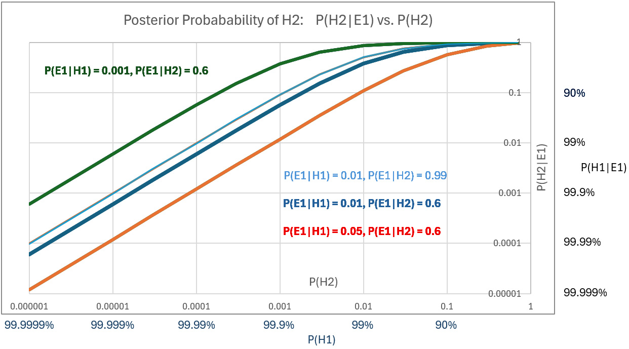
Prior hypotheses with probabilities greater the 99% represent confidence levels that are rarely justified. Nevertheless, we plot high posteriors for priors of H1 (i.e., posteriors of H2 down to 0.00001 (1E-5). Using P(E1|H1) = 0.05 and P(E1|H2 = 0.6, we get a posterior P(H2|E1) = 0.0001 – or P(H1|E1) = 99.99%, which might be initially judged as not supporting incarceration of US citizens in what were effectively concentration camps.
Risk
While there is no evidence of either explicit Bayesian reasoning or risk quantification by Franklin D. Roosevelt or military analysts, we can examine their decisions using reasonable ranges of numerical values that would have been used if numerical analysis had been employed.
We can model risk, as is common in military analysis, by defining it as the product of severity and probability – probability equal to that calculated as the posterior probability that a threat existed in the population of 120,000 who were interned.
Having established a range of probabilities for threat events above, we can now estimate severity – the cost of a loss – based on lost lives and lost defense capability resulting from a threat brought to life.
The Pearl Harbor attack itself tells us what a potential hazard might look like. Eight U.S. Navy battleships were at Pearl Harbor: Arizona, Oklahoma, West Virginia, California, Nevada, Tennessee, Maryland, and Pennsylvania. Typical peacetime crew sizes ranged from 1,200 to 1,500 per battleship, though wartime complements could exceed that. About 8,000–10,000 sailors were assigned to the battleships. More sailors would have been on board had the attack not happened on a Sunday morning.
About 37,000 Navy and 14,000 Army personnel were stationed at Pearl Harbor. 2,403 were killed in the attack, most of them aboard battleships. Four battleships were sunk. The Arizona suffered a catastrophic magazine explosion from a direct bomb hit. Over 1,170 crew members were killed. 400 were killed on the Oklahoma when it sank. None of the three aircraft carriers of the Pacific Fleet were in Pearl Harbor on Dec. 7. The USS Enterprise was due to be in port on Dec. 6 but was delayed by weather. Its crew was about 2,300 men.
Had circumstances differed slightly, the attack would not have been a surprise, and casualties would have been fewer. But in other conceivable turns of events, they could have been far greater. A modern impact analysis of an attack on Pearl Harbor or other bases would consider an invasion’s “cost” to be 10 to 20,000 lives and the loss of defense capability due to destroyed ships and aircraft. Better weather could have meant destruction of one third of US aircraft carriers in the Pacific.
Using a linear risk model, an analyst, if such analysis was done back then, might have used the above calculated P(H2|E1) as the probability of loss and 10,000 lives as one cost of the espionage. Using probability P(H1) in the range of 99.99% confidence in loyalty – i.e., P(H2) = 1E-4 – and severity = 10,000 lives yields quantified risk.
As a 1941 risk analyst, you would be considering a one-in-10,000 chance of losing 10,000 lives and loss of maybe 25% of US defense capacity. Another view of the risk would be that each of 120,000 Japanese Americans poses a one-in-10,000 chance of causing 10,000 deaths, an expected cost of roughly 120,000 lives (roughly, because the math isn’t quite as direct as it looks in this example).
While I’ve modeled the decision using a linear expected value approach, it’s important to note that real-world policy, especially in safety-critical domains, is rarely risk-neutral. For instance, Federal Aviation Regulation AC 25.1309 states that “no single failure, regardless of probability, shall result in a catastrophic condition”, a clear example of a threshold risk model overriding probabilistic reasoning. In national defense or public safety, similar thinking applies. A leader might deem a one-in-10,000 chance of catastrophic loss (say, 10,000 deaths and 25% loss of Pacific Fleet capability) intolerable, even if the expected value (loss) were only one life. This is not strictly about math; it reflects public psychology and political reality. A risk-averse or ambiguity-intolerant government could rationally act under such assumptions.
Would you take that risk, or would you incarcerate? Would your answer change if you used P(H1) = 99.999 percent? Could a prior of that magnitude ever be justified?
From the perspective of quantified risk analysis (as laid out in documents like FAR AC 25.1309), President Roosevelt, acting in early 1942 would have been justified even if P(H1) had been 99.999%.
In a society so loudly committed to consequentialist reasoning, this choice ought to seem defensible. That it doesn’t may reveal more about our moral bookkeeping than about Roosevelt’s logic. Racism existed in California in 1941, but it unlikely increased scrutiny by spy watchers. The fact that prejudice existed does not bear on the decision, because the prejudice did not motivate any action that would have born – beyond the Munson Report – on the prior probabilities used. That the Japanese Americans were held far too long is irrelevant to Roosevelt’s decision.
Since the rationality of Roosevelt’s decision, as modeled by Bayesian reasoning and quantified risk, ultimately hinges on P(H1), and since H1’s primary input was the Munson Report, we might scrutinize the way the Munson Report informs H1.
The Munson Report is often summarized with its most quoted line: “There is no Japanese ‘problem’ on the Coast.” And that was indeed its primary conclusion. Munson found Japanese American citizens broadly loyal and recommended against mass incarceration. However, if we assume the report to be wholly credible – our only source of empirical grounding at the time – then certain passages remain relevant for establishing a prior. Munson warned of possible sabotage by Japanese nationals and acknowledged the existence of a few “fanatical” individuals willing to act violently on Japan’s behalf. He recommended federal control over Japanese-owned property and proposed using loyal Nisei to monitor potentially disloyal relatives. These were not the report’s focus, but they were part of it. Critics often accuse John Franklin Carter of distorting Munson’s message when advising Roosevelt. Carter’s motives are beside the point. Whether his selective quotations were the product of prejudice or caution, the statements he cited were in the report. Even if we accept Munson’s assessment in full – affirming the loyalty of Japanese American citizens and acknowledging only rare threats – the two qualifiers Carter cited are enough to undercut extreme confidence. In modern Bayesian practice, priors above 99.999% are virtually unheard of, even in high-certainty domains like particle physics and medical diagnostics. From a decision-theoretic standpoint, Munson’s own language renders such priors unjustifiable. With confidence lower than that, Roosevelt made the rational decision – clear in its logic, devastating in its consequences.
Bayes Theorem, Pearl Harbor, and the Niihau Incident
Posted by Bill Storage in Probability and Risk on July 2, 2025
The Niihau Incident of December 7–13, 1941 provides a good case study for applying Bayesian reasoning to historical events, particularly in assessing decision-making under uncertainty. Bayesian reasoning involves updating probabilities based on new evidence, using Bayes’ theorem: P(A∣B) = P(B∣A) ⋅ P(A)P(B) / P(A|B), where:
- P(E∣H) is the likelihood of observing E given H
- P(H∣E) is the posterior probability of hypothesis H given evidence E
- P(H) is the prior probability of H
- P(E) is the marginal probability of E.
Terms like P(E∣H), the probability of evidence given a hypothesis, can be confusing. Alternative phrasings may help:
- The probability of observing evidence E if hypothesis H were true
- The likelihood of E given H
- The conditional probability of E under H
These variations clarify that we’re assessing how likely the evidence is under a specific scenario, not the probability of the hypothesis itself, which is P(H∣E).
In the context of the Niihau Incident, we can use Bayesian reasoning to analyze the decisions made by the island’s residents, particularly the Native Hawaiians and the Harada family, in response to the crash-landing of Japanese pilot Shigenori Nishikaichi. Below, I’ll break down the analysis, focusing on key decisions and quantifying probabilities while acknowledging the limitations of historical data.
Context of the Niihau Incident
On December 7, 1941, after participating in the Pearl Harbor attack, Japanese pilot Shigenori Nishikaichi crash-landed his damaged A6M2 Zero aircraft on Niihau, a privately owned Hawaiian island with a population of 136, mostly Native Hawaiians. The Japanese Navy had mistakenly designated Niihau as an uninhabited island for emergency landings, expecting pilots to await rescue there. The residents, unaware of the Pearl Harbor attack, initially treated Nishikaichi as a guest but confiscating his weapons. Over the next few days, tensions escalated as Nishikaichi, with the help of Yoshio Harada and his wife Irene, attempted to destroy his plane and papers, took hostages, and engaged in violence. The incident culminated in the Kanaheles, a Hawaiian couple, overpowering and killing Nishikaichi. Yoshio Harada committing suicide.
From a Bayesian perspective, we can analyze the residents updating their beliefs as new evidence emerged.
We define two primary hypotheses regarding Nishikaichi’s intentions:
- H1: Nishikaichi is a neutral (non-threatening) lost pilot needing assistance.
- H2: Nishikaichi is an enemy combatant with hostile intentions.
The residents’ decisions reflect the updating of beliefs about (credence in) these hypotheses.
Prior Probabilities
At the outset, the residents had no knowledge of the Pearl Harbor attack. Thus, their prior probability for P(H1) (Nishikaichi is non-threatening) would likely be high, as a crash-landed pilot could reasonably be seen as a distressed individual. Conversely, P(H2) (Nishikaichi is a threat) would be low due to the lack of context about the war.
We can assign initial priors based on this context:
- P(H1) = 0.9: The residents initially assume Nishikaichi is a non-threatening guest, given their cultural emphasis on hospitality and lack of information about the attack.
- P(H2) = 0.1: The possibility of hostility exists but is less likely without evidence of war.
These priors are subjective, reflecting the residents’ initial state of knowledge, consistent with the Bayesian interpretation of probability as a degree of belief.
We identify key pieces of evidence that influenced the residents’ beliefs:
E1: Nishikaichi’s Crash-Landing and Initial Behavior
Nishikaichi crash-landed in a field near Hawila Kaleohano, who disarmed him and treated him as a guest. His initial behavior (not hostile) supports H1.
Likelihoods:
- P(E1∣H1) = 0.95: A non-threatening pilot is highly likely to crash-land and appear cooperative.
- P(E1∣H2) = 0.3: A hostile pilot could be expected to act more aggressively, though deception is possible.
Posterior Calculation:
P(H1∣E1) = [P(E1∣H1)⋅P(H1)] / [P(E1∣H1)⋅P(H1) + P(E1∣H2)⋅P(H2) ]
P(H1|E1) = 0.95⋅0.9 / [(0.95⋅0.9) + (0.3⋅0.1)] = 0.97
After the crash, the residents’ belief in H1 justifies hospitality.
E2: News of the Pearl Harbor Attack
That night, the residents learned of the Pearl Harbor attack via radio, revealing Japan’s aggression. This significantly increases the likelihood that Nishikaichi was a threat.
Likelihoods:
- P(E2∣H1) = 0.1 P(E2|H1) = 0.1 P(E2∣H1) = 0.1: A non-threatening pilot is unlikely to be associated with a surprise attack.
- P(E2∣H2) = 0.9 P(E2|H2) = 0.9 P(E2∣H2) = 0.9: A hostile pilot is highly likely to be linked to the attack.
Posterior Calculation (using updated priors from E1):
P(H1∣E2) = P(E2∣H1)⋅P(H1∣E1) / [P(E2∣H1)⋅P(H1∣E1) + P(E2∣H2)⋅P(H2∣E1)]
P(H1∣E2) = 0.1⋅0.97 / [(0.1⋅0.97) + (0.9⋅0.03)] = 0.76
P(H2∣E2) = 0.24
The news shifts the probability toward H2, prompting the residents to apprehend Nishikaichi and put him under guard with the Haradas.
E3: Nishikaichi’s Collusion with the Haradas
Nishikaichi convinced Yoshio and Irene Harada to help him escape, destroy his plane, and burn Kaleohano’s house to eliminate his papers.
Likelihoods:
- P(E3∣H1) = 0.01: A non-threatening pilot is extremely unlikely to do this.
- P(E3∣H2) = 0.95: A hostile pilot is likely to attempt to destroy evidence and escape.
Posterior Calculation (using updated priors from E2):
P(H1∣E3) = P(E3∣H1)⋅P(H1∣E2) / [P(E3∣H1)⋅P(H1∣E2) + P(E3∣H2)⋅P(H2∣E2)]
P(H1∣E3) = 0.01⋅0.759 / [(0.01⋅0.759) + (0.95⋅0.241)] = 0.032
P(H2∣E3) = 0.968
This evidence dramatically increases the probability of H2, aligning with the residents’ decision to confront Nishikaichi.
E4: Nishikaichi Takes Hostages and Engages in Violence
Nishikaichi and Harada took Ben and Ella Kanahele hostage, and Nishikaichi fired a machine gun. Hostile intent is confirmed.
Likelihoods:
- P(E4∣H1) = 0.001: A non-threatening pilot is virtually certain not to take hostages or use weapons.
- P(E4∣H2) = 0.99: A hostile pilot is extremely likely to resort to violence.
Posterior Calculation (using updated priors from E3):
P(H1∣E4) = P(E4∣H1)⋅P(H1∣E3)/ [P(E4∣H1)⋅P(H1∣E3) + P(E4∣H2)⋅P(H2∣E3)P(H1|E4)]
P(H1∣E4) = 0.001⋅0.032 / [(0.001⋅0.032)+(0.99⋅0.968)] =0.00003
P(H2∣E4) = 1.0 – P(H1∣E4) = 0.99997
At this point, the residents’ belief in H2 is near certainty, justifying the Kanaheles’ decisive action to overpower Nishikaichi.
Uncertainty Quantification
Bayesian reasoning also involves quantifying uncertainty, particularly aleatoric (inherent randomness) and epistemic (model uncertainty) components.
Aleatoric Uncertainty: The randomness in Nishikaichi’s actions (e.g., whether he would escalate to violence) was initially high due to the residents’ lack of context. As evidence accumulated, this uncertainty decreased, as seen in the near-certain posterior for H2 after E4.
Epistemic Uncertainty: The residents’ model of Nishikaichi’s intentions was initially flawed due to their isolation and lack of knowledge about the war. This uncertainty reduced as they incorporated news of Pearl Harbor and observed Nishikaichi’s actions, refining their model of his behavior.
Analysis of Decision-Making
The residents’ actions align with Bayesian updating:
Initial Hospitality (E1): High prior for H1 led to treating Nishikaichi as a guest, with precautions (disarming him) reflecting slight uncertainty.
Apprehension (E2): News of Pearl Harbor shifted probabilities toward H2, prompting guards and confinement with the Haradas.
Confrontations (E3, E4): Nishikaichi’s hostile actions (collusion, hostage-taking) pushed P(H2) to near 1, leading to the Kanaheles’ lethal response.
The Haradas’ decision to assist Nishikaichi complicates the analysis. Their priors may have been influenced by cultural or personal ties to Japan, increasing their P(H1) or introducing a separate hypothesis of loyalty to Japan. Lack of detailed psychological data makes quantifying their reasoning speculative.
Limitations and Assumptions
Subjective Priors: The assigned priors (e.g., P(H1) = 0.9) are estimates based on historical context, not precise measurements. Bayesian reasoning allows subjective priors, but different assumptions could alter results.
Likelihood Estimates: Likelihoods (e.g., P(E1∣H1) = 0.95) are informed guesses, as historical records lack data on residents’ perceptions.
Simplified Hypotheses: I used two hypotheses for simplicity. In reality, residents may have considered nuanced possibilities, e.g., Nishikaichi being coerced or acting out of desperation.
Historical Bias: may exaggerate or omit details, affecting our understanding of evidence.
Conclusion
Bayesian reasoning (Subjective Bayes) provides a structured framework to understand how Niihau’s residents updated their beliefs about Nishikaichi’s intentions. Initially, a high prior for him being non-threatening (P(H1)=0.9) was reasonable given their isolation. As evidence accumulated (news of Pearl Harbor, Nishikaichi’s collusion with the Haradas, and his violent actions) the posterior probability of hostility, P(H2) approached certainty, justifying their escalating responses. Quantifying this process highlights the rationality of their decisions under uncertainty, despite limited information. This analysis demonstrates Bayesian inference used to model historical decision-making, assuming the deciders were rational agents.
Next
The Niihau Incident influenced U.S. policy decisions regarding the internment of Japanese Americans during World War II. It heightened fears of disloyalty among Japanese Americans. Applying Bayesian reasoning to the decision to intern Japanese Americans after the Niihau Incident might provide insight on how policymakers updated their beliefs about the potential threat posed by this population based on limited evidence and priors. In a future post, I’ll use Bayes’ theorem to model this decision-making process to model the quantification of risk.
Statistical Reasoning in Healthcare: Lessons from Covid-19
Posted by Bill Storage in History of Science, Philosophy of Science, Probability and Risk on May 6, 2025
For centuries, medicine has navigated the tension between science and uncertainty. The Covid pandemic exposed this dynamic vividly, revealing both the limits and possibilities of statistical reasoning. From diagnostic errors to vaccine communication, the crisis showed that statistics is not just a technical skill but a philosophical challenge, shaping what counts as knowledge, how certainty is conveyed, and who society trusts.
Historical Blind Spot
Medicine’s struggle with uncertainty has deep roots. In antiquity, Galen’s reliance on reasoning over empirical testing set a precedent for overconfidence insulated by circular logic. If his treatments failed, it was because the patient was incurable. Enlightenment physicians, like those who bled George Washington to death, perpetuated this resistance to scrutiny. Voltaire wrote, “The art of medicine consists in amusing the patient while nature cures the disease.” The scientific revolution and the Enlightenment inverted Galen’s hierarchy, yet the importance of that reversal is often neglected, even by practitioners. Even in the 20th century, pioneers like Ernest Codman faced ostracism for advocating outcome tracking, highlighting a medical culture that prized prestige over evidence. While evidence-based practice has since gained traction, a statistical blind spot persists, rooted in training and tradition.
The Statistical Challenge
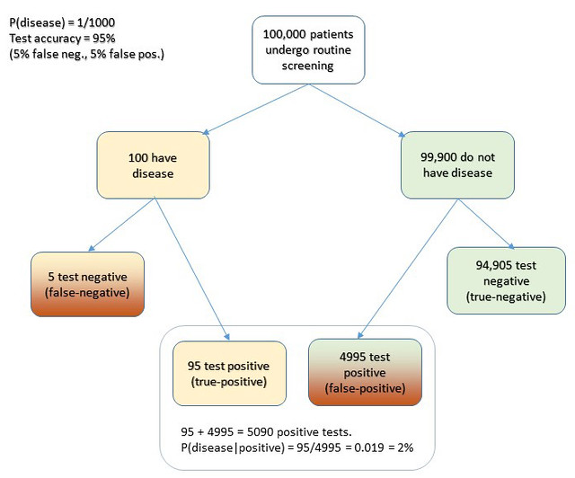
Physicians often struggle with probabilistic reasoning, as shown in a 1978 Harvard study where only 18% correctly applied Bayes’ Theorem to a diagnostic test scenario (a disease with 1/1,000 prevalence and a 5% false positive rate yields a ~2% chance of disease given a positive test). A 2013 follow-up showed marginal improvement (23% correct). Medical education, which prioritizes biochemistry over probability, is partly to blame. Abusive lawsuits, cultural pressures for decisiveness, and patient demands for certainty further discourage embracing doubt, as Daniel Kahneman’s work on overconfidence suggests.
Neil Ferguson and the Authority of Statistical Models
Epidemiologist Neil Ferguson and his team at Imperial College London produced a model in March 2020 predicting up to 500,000 UK deaths without intervention. The US figure could top 2 million. These weren’t forecasts in the strict sense but scenario models, conditional on various assumptions about disease spread and response.
Ferguson’s model was extraordinarily influential, shifting the UK and US from containment to lockdown strategies. It also drew criticism for opaque code, unverified assumptions, and the sheer weight of its political influence. His eventual resignation from the UK’s Scientific Advisory Group for Emergencies (SAGE) over a personal lockdown violation further politicized the science.
From the perspective of history of science, Ferguson’s case raises critical questions: When is a model scientific enough to guide policy? How do we weigh expert uncertainty under crisis? Ferguson’s case shows that modeling straddles a line between science and advocacy. It is, in Kuhnian terms, value-laden theory.
The Pandemic as a Pedagogical Mirror
The pandemic was a crucible for statistical reasoning. Successes included the clear communication of mRNA vaccine efficacy (95% relative risk reduction) and data-driven ICU triage using the SOFA score, though both had limitations. Failures were stark: clinicians misread PCR test results by ignoring pre-test probability, echoing the Harvard study’s findings, while policymakers fixated on case counts over deaths per capita. The “6-foot rule,” based on outdated droplet models, persisted despite disconfirming evidence, reflecting resistance to updating models, inability to apply statistical insights, and institutional inertia. Specifics of these issues are revealing.
Mostly Positive Examples:
- Risk Communication in Vaccine Trials (1)
The early mRNA vaccine announcements in 2020 offered clear statistical framing by emphasizing a 95% relative risk reduction in symptomatic COVID-19 for vaccinated individuals compared to placebo, sidelining raw case counts for a punchy headline. While clearer than many public health campaigns, this focus omitted absolute risk reduction and uncertainties about asymptomatic spread, falling short of the full precision needed to avoid misinterpretation. - Clinical Triage via Quantitative Models (2)
During peak ICU shortages, hospitals adopted the SOFA score, originally a tool for assessing organ dysfunction, to guide resource allocation with a semi-objective, data-driven approach. While an improvement over ad hoc clinical judgment, SOFA faced challenges like inconsistent application and biases that disadvantaged older or chronically ill patients, limiting its ability to achieve fully equitable triage. - Wastewater Epidemiology (3)
Public health researchers used viral RNA in wastewater to monitor community spread, reducing the sampling biases of clinical testing. This statistical surveillance, conducted outside clinics, offered high public health relevance but faced biases and interpretive challenges that tempered its precision.
Mostly Negative Examples:
- Misinterpretation of Test Results (4)
Early in the COVID-19 pandemic, many clinicians and media figures misunderstood diagnostic test accuracy, misreading PCR and antigen test results by overlooking pre-test probability. This caused false reassurance or unwarranted alarm, though some experts mitigated errors with Bayesian reasoning. This was precisely the type of mistake highlighted in the Harvard study decades earlier. - Cases vs. Deaths (5)
One of the most persistent statistical missteps during the pandemic was the policy focus on case counts, devoid of context. Case numbers ballooned or dipped not only due to viral spread but due to shifts in testing volume, availability, and policies. COVID deaths per capita rather than case count would have served as a more stable measure of public health impact. Infection fatality rates would have been better still. - Shifting Guidelines and Aerosol Transmission (6)
The “6-foot rule” was based on outdated models of droplet transmission. When evidence of aerosol spread emerged, guidance failed to adapt. Critics pointed out the statistical conservatism in risk modeling, its impact on mental health and the economy. Institutional inertia and politics prevented vital course corrections.
(I’ll defend these six examples in another post.)
A Philosophical Reckoning
Statistical reasoning is not just a mathematical tool – it’s a window into how science progresses, how it builds trust, and its special epistemic status. In Kuhnian terms, the pandemic exposed the fragility of our current normal science. We should expect methodological chaos and pluralism within medical knowledge-making. Science during COVID-19 was messy, iterative, and often uncertain – and that’s in some ways just how science works.
This doesn’t excuse failures in statistical reasoning. It suggests that training in medicine should not only include formal biostatistics, but also an eye toward history of science – so future clinicians understand the ways that doubt, revision, and context are intrinsic to knowledge.
A Path Forward
Medical education must evolve. First, integrate Bayesian philosophy into clinical training, using relatable case studies to teach probabilistic thinking. Second, foster epistemic humility, framing uncertainty as a strength rather than a flaw. Third, incorporate the history of science – figures like Codman and Cochrane – to contextualize medicine’s empirical evolution. These steps can equip physicians to navigate uncertainty and communicate it effectively.
Conclusion
Covid was a lesson in the fragility and potential of statistical reasoning. It revealed medicine’s statistical struggles while highlighting its capacity for progress. By training physicians to think probabilistically, embrace doubt, and learn from history, medicine can better manage uncertainty – not as a liability, but as a cornerstone of responsible science. As John Heilbron might say, medicine’s future depends not only on better data – but on better historical memory, and the nerve to rethink what counts as knowledge.
______
All who drink of this treatment recover in a short time, except those whom it does not help, all of whom die. It is obvious, therefore, that it fails only in incurable cases. – Galen
The Prosecutor’s Fallacy Illustrated
Posted by Bill Storage in Probability and Risk on May 7, 2020
“The first thing we do, let’s kill all the lawyers.” – Shakespeare, Henry VI, Part 2, Act IV
My last post discussed the failure of most physicians to infer the chance a patient has the disease given a positive test result where both the frequency of the disease in the population and the accuracy of the diagnostic test are known. The probability that the patient has the disease can be hundreds or thousands of times lower than the accuracy of the test. The problem in reasoning that leads us to confuse these very different likelihoods is one of several errors in logic commonly called the prosecutor’s fallacy. The important concept is conditional probability. By that we mean simply that the probability of x has a value and that the probability of x given that y is true has a different value. The shorthand for probability of x is p(x) and the shorthand for probability of x given y is p(x|y).
“Punching, pushing and slapping is a prelude to murder,” said prosecutor Scott Gordon during the trial of OJ Simpson for the murder of Nicole Brown. Alan Dershowitz countered with the argument that the probability of domestic violence leading to murder was very remote. Dershowitz (not prosecutor but defense advisor in this case) was right, technically speaking. But he was either as ignorant as the physicians interpreting the lab results or was giving a dishonest argument, or possibly both. The relevant probability was not the likelihood of murder given domestic violence, it was the likelihood of murder given domestic violence and murder. “The courtroom oath – to tell the truth, the whole truth and nothing but the truth – is applicable only to witnesses,” said Dershowitz in The Best Defense. In Innumeracy: Mathematical Illiteracy and Its Consequences. John Allen Paulos called Dershowitz’s point “astonishingly irrelevant,” noting that utter ignorance about probability and risk “plagues far too many otherwise knowledgeable citizens.” Indeed.
The doctors’ mistake in my previous post was confusing
P(positive test result) vs.
P(disease | positive test result)
Dershowitz’s argument confused
P(husband killed wife | husband battered wife) vs.
P(husband killed wife | husband battered wife | wife was killed)
In Reckoning With Risk, Gerd Gigerenzer gave a 90% value for the latter Simpson probability. What Dershowitz cited was the former, which we can estimate at 0.1%, given a wife-battery rate of one in ten, and wife-murder rate of one per hundred thousand. So, contrary to what Dershowitz implied, prior battery is a strong indicator of guilt when a wife has been murdered.
As mentioned in the previous post, the relevant mathematical rule does not involve advanced math. It’s a simple equation due to Pierre-Simon Laplace, known, oddly, as Bayes’ Theorem:
P(A|B) = P(B|A) * P(A) / P(B)
If we label the hypothesis (patient has disease) as D and the test data as T, the useful form of Bayes’ Theorem is
P(D|T) = P(T|D) P(D) / P(T) where P(T) is the sum of probabilities of positive results, e.g.,
P(T) = P(T|D) * P(D) + P(T | not D) * P(not D) [using “not D” to mean “not diseased”]
Cascells’ phrasing of his Harvard quiz was as follows: “If a test to detect a disease whose prevalence is 1 out of 1,000 has a false positive rate of 5 percent, what is the chance that a person found to have a positive result actually has the disease?”
Plugging in the numbers from the Cascells experiment (with the parameters Cascells provided shown below in bold and the correct answer in green):
- P(D) is the disease frequency = 0.001 [ 1 per 1000 in population ] therefore:
- P(not D) is 1 – P(D) = 0.999
- P(T | not D) = 5% = 0.05 [ false positive rate also 5%] therefore:
- P(T | D) = 95% = 0.95 [ i.e, the false negative rate is 5% ]
Substituting:
P(T) = .95 * .001 + .999 * .05 = 0.0509 ≈ 5.1% [ total probability of a positive test ]
P(D|T) = .95 * .001 / .0509 = .0019 ≈ 2% [ probability that patient has disease, given a positive test result ]
Voila.
I hope this seeing is believing illustration of Cascells’ experiment drives the point home for those still uneasy with equations. I used Cascells’ rates and a population of 100,000 to avoid dealing with fractional people:
Extra credit: how exactly does this apply to Covid, news junkies?
Edit 5/21/20. An astute reader called me on an inaccuracy in the diagram. I used an approximation, without identifying it. P = r1/r2 is a cheat for P = 1 – Exp(- r1/r2). The approximation is more intuitive, though technically wrong. It’s a good cheat, for P values less that 10%.
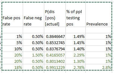
Note 5/22/20. In response to questions about how this sort of thinking bears on coronavirus testing -what test results say about prevalence – consider this. We really have one equation in 3 unknowns here: false positive rate, false negative rate, and prevalence in population. A quick Excel variations study using false positive rates from 1 to 20% and false neg rates from 1 to 3 percent, based on a quick web search for proposed sensitivity/specificity for the Covid tests is revealing. Taking the low side of the raw positive rates from the published data (1 – 3%) results in projected prevalence roughly equal to the raw positive rates. I.e., the false positives and false negatives happen to roughly wash out in this case. That also leaves P(d|t) in the range of a few percent.
The Trouble with Doomsday
Posted by Bill Storage in Philosophy, Probability and Risk on February 4, 2020
Doomsday just isn’t what is used to be. Once the dominion of ancient apologists and their votary, the final destiny of humankind now consumes probability theorists, physicists. and technology luminaries. I’ll give some thoughts on probabilistic aspects of the doomsday argument after a brief comparison of ancient and modern apocalypticism.
Apocalypse Then
The Israelites were enamored by eschatology. “The Lord is going to lay waste the earth and devastate it,” wrote Isaiah, giving few clues about when the wasting would come. The early Christians anticipated and imminent end of days. Matthew 16:27: some of those who are standing here will not taste death until they see the Son of Man coming in His kingdom.
From late antiquity through the middle ages, preoccupation with the Book of Revelation led to conflicting ideas about the finer points of “domesday,” as it was called in Middle English. The first millennium brought a flood of predictions of, well, flood, along with earthquakes, zombies, lakes of fire and more. But a central Christian apocalyptic core was always beneath these varied predictions.
Right up to the enlightenment, punishment awaited the unrepentant in a final judgment that, despite Matthew’s undue haste, was still thought to arrive any day now. Disputes raged over whether the rapture would be precede the tribulation or would follow it, the proponents of each view armed with supporting scripture. Polarization! When Christianity began to lose command of its unruly flock in the 1800’s, Nietzsche wondered just what a society of non-believers would find to flog itself about. If only he could see us now.
Apocalypse Now
Our modern doomsday riches include options that would turn an ancient doomsayer green. Alas, at this eleventh hour we know nature’s annihilatory whims, including global pandemic, supervolcanoes, asteroids, and killer comets. Still in the Acts of God department, more learned handwringers can sweat about earth orbit instability, gamma ray bursts from nearby supernovae, or even a fluctuation in the Higgs field that evaporates the entire universe.
As Stephen Hawking explained bubble nucleation, the Higgs field might be metastable at energies above a certain value, causing a region of false vacuum to undergo catastrophic vacuum decay, causing a bubble of the true vacuum expanding at the speed of light. This might have started eons ago, arriving at your doorstep before you finish this paragraph. Harold Camping, eat your heart out.
Hawking also feared extraterrestrial invasion, a view hard to justify with probabilistic analyses. Glorious as such cataclysms are, they lack any element of contrition. Real apocalypticism needs a guilty party.
Thus anthropogenic climate change reigned for two decades with no creditable competitors. As self-inflicted catastrophes go, it had something for everyone. Almost everyone. Verily, even Pope Francis, in a covenant that astonished adherents, joined – with strong hand and outstretched arm – leftists like Naomi Oreskes, who shares little else with the Vatican, ideologically speaking.
While Global Warming is still revered, some prophets now extend the hand of fellowship to some budding successor fears, still tied to devilries like capitalism and the snare of scientific curiosity. Bioengineered coronaviruses might be invading as we speak. Careless researchers at the Large Hadron Collider could set off a mini black hole that swallows the earth. So some think anyway.
Nanotechnology now gives some prominent intellects the willies too. My favorite in this realm is Gray Goo, a catastrophic chain of events involving molecular nanobots programmed for self-replication. They will devour all life and raw materials at an ever-increasing rate. How they’ll manage this without melting themselves due to the normal exothermic reactions tied to such processes is beyond me. Global Warming activists may become jealous, as the very green Prince Charles himself now diverts a portion of the crown’s royal dread to this upstart alternative apocalypse.
My cataclysm bucks are on full-sized Artificial Intelligence though. I stand with chief worriers Bill Gates, Ray Kurzweil, and Elon Musk. Computer robots will invent and program smarter and more ruthless autonomous computer robots on a rampage against humans seen by the robots as obstacles to their important business of building even smarter robots. Game over.
The Mathematics of Doomsday
The Doomsday Argument is a mathematical proposition arising from the Copernican principle – a trivial application of Bayesian reasoning – wherein we assume that, lacking other info, we should find ourselves, roughly speaking, in the middle of the phenomenon of interest. Copernicus didn’t really hold this view, but 20th century thinkers blamed him for it anyway.
Applying the Copernican principle to human life starts with the knowledge that we’ve been around for 200 hundred thousand years, during which 60 billion of us have lived. Copernicans then justify the belief that half the humans that will have ever lived remain to be born. With an expected peak earth population of 12 billion, we might, using this line of calculating, expect the human race to go extinct in a thousand years or less.
Adding a pinch of statistical rigor, some doomsday theorists calculate a 95% probability that the number of humans to have lived so far is less than 20 times the number that will ever live. Positing individual life expectancy of 100 years and 12 billion occupants, the earth will house humans for no more than 10,000 more years.
That’s the gist of the dominant doomsday argument. Notice that it is purely probabilistic. It applies equally to the Second Coming and to Gray Goo. However, its math and logic are both controversial. Further, I’m not sure why its proponents favor population-based estimates over time-based estimates. That is, it took a lot longer than 10,000 years, the proposed P = .95 extinction term, for the race to arrive at our present population. So why not place the current era in the middle of the duration of the human race, thereby giving us another 200,000 thousand years? That’s quite an improvement on the 10,000 year prediction above.
Even granting that improvement, all the above doomsday logic has some curious bugs. If we’re justified in concluding that we’re midway through our reign on earth, then should we also conclude we’re midway through the existence of agriculture and cities? If so, given that cities and agriculture emerged 10,000 years ago, we’re led to predict a future where cities and agriculture disappear in 10,000 years, followed by 190,000 years of post-agriculture hunter-gatherers. Seems unlikely.
Astute Bayesian reasoners might argue that all of the above logic relies – unjustifiably – on an uninformative prior. But we have prior knowledge suggesting we don’t happen to be at some random point in the life of mankind. Unfortunately, we can’t agree on which direction that skews the outcome. My reading of the evidence leads me to conclude we’re among the first in a long line of civilized people. I don’t share Elon Musk’s pessimism about killer AI. And I find Hawking’s extraterrestrial worries as facile as the anti-GMO rantings of the Union of Concerned Scientists. You might read the evidence differently. Others discount the evidence altogether, and are simply swayed by the fashionable pessimism of the day.
Finally, the above doomsday arguments all assume that we, as observers, are randomly selected from the set of all existing humans, including past, present and future, ever be born, as opposed to being selected from all possible births. That may seem a trivial distinction, but, on close inspection, becomes profound. The former is analogous to Theory 2 in my previous post, The Trouble with Probability. This particular observer effect, first described by Dennis Dieks in 1992, is called the self-sampling assumption by Nick Bostrom. Considering yourself to be randomly selected from all possible births prior to human extinction is the analog of Theory 3 in my last post. It arose from an equally valid assumption about sampling. That assumption, called self-indication by Bostrom, confounds the above doomsday reasoning as it did the hotel problem in the last post.
Th self-indication assumption holds that we should believe that we’re more likely to discover ourselves to be members of larger sets than of smaller sets. As with the hotel room problem discussed last time, self-indication essentially cancels out the self-sampling assumption. We’re more likely to be in a long-lived human race than a short one. In fact, setting aside some secondary effects, we can say that the likelihood of being selected into any set is proportional to the size of the set; and here we are in the only set we know of. Doomsday hasn’t been called off, but it has been postponed indefinitely.
The Trouble with Probability
Posted by Bill Storage in Probability and Risk on February 2, 2020
The trouble with probability is that no one agrees what it means.
Most people understand probability to be about predicting the future and statistics to be about the frequency of past events. While everyone agrees that probability and statistics should have something to do with each other, no one agrees on what that something is.
Probability got a rough start in the world of math. There was no concept of probability as a discipline until about 1650 – odd, given that gambling had been around for eons. Some of the first serious work on probability was done by Blaise Pascal, who was assigned by a nobleman to divide up the winnings when a dice game ended unexpectedly. Before that, people just figured chance wasn’t receptive to analysis. Aristotle’s idea of knowledge required that it be universal and certain. Probability didn’t fit.
To see how fast the concept of probability can go haywire, consider your chance of getting lung cancer. Most agree that probability is determined by your membership in a reference class for which a historical frequency is known. Exactly which reference class you belong to is always a matter of dispute. How similar to them do you need to be? The more accurately you set the attributes of the reference population, the more you narrow it down. Eventually, you get down to people of your age, weight, gender, ethnicity, location, habits, and genetically determined preference for ice cream flavor. Your reference class then has a size of one – you. At this point your probability is either zero or one, and nothing in between. The historical frequency of cancer within this population (you) cannot predict your future likelihood of cancer. That doesn’t seem like what we wanted to get from probability.
Similarly, in the real world, the probabilities of uncommon events and of events with no historical frequency at all are the subject of keen interest. For some predictions of previously unexperienced events, like and airplane crashing due to simultaneous failure of a certain combination of parts, even though that combination may have never occurred in the past, we can assemble a probability from combining historical frequencies of the relevant parts using Boolean logic. My hero Richard Feynman seemed not to grasp this, oddly.
For worries like a large city being wiped out by an asteroid, our reasoning becomes more conjectural. But even for asteroids we can learn quite a bit about asteroid impact rates based on the details of craters on the moon, where the craters don’t weather away so fast as they do on earth. You can see that we’re moving progressively away from historical frequencies and becoming more reliant on inductive reasoning, the sort of thing that gave Aristotle the hives.
Finally, there are some events for which historical frequencies provide no useful information. The probability that nanobots will wipe out the human race, for example. In these cases we take a guess, maybe even a completely wild guess. and then, on incrementally getting tiny bits of supporting or nonsupporting evidence, we modify our beliefs. This is the realm of Bayesianism. In these cases when we talk about probability we are really only talking about the degree to which we believe a proposition, conjecture or assertion.
Breaking it down a bit more formally, a handful of related but distinct interpretations of probability emerge. Those include, for example:
Objective chances: The physics of flipping a fair coin tend to result in heads half the time.
Frequentism: Relative frequency across time: of all the coins ever flipped, one half have been heads, so expect more of the same.
Hypothetical frequentism: If you flipped coins forever, the heads/tails ratio would approach 50%.
Bayesian belief: Prior distributions equal belief: before flipping a coin, my personal expectation that it will be heads is equal to that of it being tails.
Objective Bayes: Prior distributions represent neutral knowledge: given only that a fair coin has been flipped, the plausibility of it’s having fallen heads equals that of it having been tails.
While those all might boil down to the same thing in the trivial case of a coin toss, they can differ mightily for difficult questions.
People’s ideas of probability differ more than one might think, especially when it becomes personal. To illustrate, I’ll use a problem derived from one that originated either with Nick Bostrom, Stuart Armstrong or Tomas Kopf, and was later popularized by Isaac Arthur. Suppose you wake up in a room after suffering amnesia or a particularly bad night of drinking. You find that you’re part of a strange experiment. You’re told that you’re in one of 100 rooms and that the door of your room is either red or blue. You’re instructed to guess which color it is. Finding a coin in your pocket you figure flipping it is as good a predictor of door color as anything else, regardless of the ratio of red to blue doors, which is unknown to you. Heads red, tails blue.
The experimenter then gives you new info. 90 doors are red and 10 doors are blue. Guess your door color, says the experimenter. Most people think, absent any other data, picking red is a 4 1/2 times better choice than letting a coin flip decide.
Now you learn that the evil experimenter had designed two different branches of experimentation. In Experiment A, ten people would be selected and placed, one each, into rooms 1 through 10. For Experiment B, 100 other people would be placed, one each, in all 100 rooms. You don’t know which room you’re in or which experiment, A or B, was conducted. The experimenter tells you he flipped a coin to choose between Experiment A, heads, and Experiment B, tails. He wants you to guess which experiment, A or B, won his coin toss. Again, you flip your coin to decide, as you have nothing to inform a better guess. You’re flipping a coin to guess the result of his coin flip. Your odds are 50-50. Nothing controversial so far.
Now you receive new information. You are in Room 5. What judgment do you now make about the result of his flip? Some will say that the odds of experiment A versus B were set by the experimenter’s coin flip, and are therefore 50-50. Call this Theory 1.
Others figure that your chance of being in Room 5 under Experiment A is 1 in 10 and under Experiment B is 1 in 100. Therefore it’s ten times more likely that Experiment A was the outcome of the experimenter’s flip. Call this Theory 2.
Still others (Theory 3) note that having been selected into a group of 100 was ten times more likely than having been selected into a group of 10, and on that basis it is ten times more likely that Experiment B was the result of the experimenter’s flip than Experiment A.
My experience with inflicting this problem on victims is that most people schooled in science – though certainly not all – prefer Theories 2 or 3 to Theory 1, suggesting they hold different forms of Bayesian reasoning. But between Theories 2 and 3, war breaks out.
Those preferring Theory 2 think the chance of having been selected into Experiment A (once it became the outcome of the experimenter’s coin flip) is 10 in 110 and the chance of being in Room 5 is 1 in 10, given that Experiment A occurred. Those who hold Theory 3 perceive a 100 in 110 chance of having been selected into Experiment B, once it was selected by the experimenter’s flip, and then a 1 in 100 chance of being in Room 5, given Experiment B. The final probabilities of being in room 5 under Theories 2 and 3 are equal (10/110 x 1/10 equals 1 in 110, vs. 100/110 x 1/100 also equals 1 in 110), but the answer to the question about the outcome of the experimenter’s coin flip having been heads (Experiment A) and tails (Experiment B) remains in dispute. To my knowledge, there is no basis for settling that dispute. Unlike Martin Gardner’s boy-girl paradox, this dispute does not result from ambiguous phrasing; it seems a true paradox.
The trouble with probability makes it all the more interesting. Is it math, philosophy, or psychology?
How dare we speak of the laws of chance. Is not chance the antithesis of all law? – Joseph Bertrand, Calcul des probabilités, 1889
Though there be no such thing as Chance in the world; our ignorance of the real cause of any event has the same influence on the understanding, and begets a like species of belief or opinion. – David Hume, An Enquiry Concerning Human Understanding, 1748
It is remarkable that a science which began with the consideration of games of chance should have become the most important object of human knowledge. – Blaise Pascal, Théorie Analytique des Probabilitiés, 1812
A short introduction to small data
Posted by Bill Storage in Probability and Risk on January 13, 2020
How many children are abducted each year? Did you know anyone who died in Vietnam?
Wikipedia explains that big data is about correlations, and that small data is either about the causes of effects, or is an inference from big data. None of that captures what I mean by small data.
Most people in my circles instead think small data deals with inferences about populations made from the sparse data from within those populations. For Bayesians, this means making best use of an intuitive informative prior distribution for a model. For wise non-Bayesians, it can mean bullshit detection.
In the early 90’s I taught a course on probabilistic risk analysis in aviation. In class we were discussing how to deal with estimating equipment failure rates where few previous failures were known when Todd, a friend who was attending the class, asked how many kids were abducted each year. I didn’t know. Nor did anyone else. But we all understood where Todd was going with the question.
Todd produced a newspaper clipping citing an evangelist – Billy Graham as I recall – who claimed that 50,000 children a year were abducted in the US. Todd asked if we thought that yielded a a reasonable prior distribution.
Seeing this as a sort of Fermi problem, the class kicked it around a bit. How many kids’ pictures are on milk cartons right now, someone asked (Milk Carton Kids – remember, this was pre-internet). We remembered seeing the same few pictures of missing kids on milk cartons for months. None of us knew of anyone in our social circles who had a child abducted. How does that affect your assessment of Billy Graham’s claim?
What other groups of people have 50,000 members I asked. Americans dead in Vietnam, someone said. True, about 50,000 American service men died in Vietnam (including 9000 accidents and 400 suicides, incidentally). Those deaths spanned 20 years. I asked the class if anyone had known someone, at least indirectly, who died in Vietnam (remember, this was the early 90s and most of us had once owned draft cards). Almost every hand went up. Assuming that dead soldiers and our class were roughly randomly selected implied each of our social spheres had about 4000 members (200 million Americans in 1970, divided by 50,000 deaths). That seemed reasonable, given that news of Vietnam deaths propagated through friends-of-friends channels.
Now given that most of us had been one or two degrees’ separation from someone who died in Vietnam, could Graham’s claim possibly be true? No, we reasoned, especially since news of abductions should travel through social circles as freely as Vietnam deaths. And those Vietnam deaths had spanned decades. Graham was claiming 50,000 abductions per year.
Automobile deaths, someone added. Those are certainly randomly distributed across income, class and ethnicity. Yes, and, oddly, they occur at a rate of about 50,000 per year in the US. Anyone know someone who died in a car accident? Every single person in the class did. Yet none of us had been close to an abduction. Abductions would have to be very skewed against aerospace engineers for our car death and abduction experience to be so vastly different given their supposedly equal occurrence rates in the larger population. But the Copernican position that we resided nowhere special in the landscapes of either abductions or automobile deaths had to be mostly valid, given the diversity of age, ethnicity and geography in the class (we spanned 30 years in age, with students from Washington, California and Missouri).
One way to check the veracity of Graham’s claim would have been to do a bunch of research. That would have been library slow and would have likely still required extrapolation and assumptions about distributions and the representativeness of whatever data we could dig up. Instead we drew a sound inference from very small data, our own sampling of world events.
We were able to make good judgments about the rate of abduction, which we were now confident was very, very much lower than one per thousand (50,000 abductions per year divide by 50 million kids). Our good judgments stemmed from our having rich priors (prior distributions) because we had sampled a lot of life and a lot of people. We had rich data about deaths from car wrecks and Vietnam, and about how many kids were not abducted in each of our admittedly small circles. Big data gets the headlines, causing many of us to forget just how good small data can be.
Use and Abuse of Failure Mode & Effects Analysis in Business
Posted by Bill Storage in Management Science, Probability and Risk on December 5, 2019
On investigating about 80 deaths associated with the drug heparin in 2009, the FDA found that over-sulphated chondroitin with toxic effects had been intentionally substituted for a legitimate ingredient for economic reasons. That is, an unscrupulous supplier sold a counterfeit chemical costing 1% as much as the real thing and it killed people.
This wasn’t unprecedented. Gentamicin, in the late 1980s, was a similar case. Likewise Cefaclor in 1996, and again with diethylene glycol sold as glycerin in 2006.
Adulteration is an obvious failure mode of supply chains and operations for drug makers. Drug firms buying adulterated raw material had presumably conducted failure mode effects analyses at several levels. An early-stage FMEA should have seen the failure mode and assessed its effects, thereby triggering the creation of controls to prevent the process failure. So what went wrong?
The FDA’s reports on the heparin incident didn’t make public any analyses done by the drug makers. But based on the “best practices” specified by standards bodies, consulting firms, and many risk managers, we can make a good guess. Their risk assessments were likely misguided, poorly executed, gutless, and ineffective.
 Promoters of FMEAs as a means of risk analysis often cite aerospace as a guiding light in matters of risk. Commercial aviation should be the exemplar of risk management. In no other endeavor has mankind made such an inherently dangerous activity so safe as commercial jet flight.
While those in pharmaceutical risk and compliance extol aviation, they mostly stray far from its methods, mindset, and values. This is certainly the case with the FMEA, a tool poorly understood, misapplied, poorly executed, and then blamed for failing to prevent catastrophe.
In the case of heparin, a properly performed FMEA exercise would certainly have identified the failure mode. But FMEA wasn’t even the right tool for identifying that hazard in the first place. A functional hazard anlysis (FHA) or Business Impact Analysis (BIA) would have highlighted chemical contamination leading to death of patients, supply disruption, and reputation damage as a top hazard in minutes. I know this for fact, because I use drug manufacture as an example when teaching classes on FHA. First-day students identify that hazard without being coached.
FHAs can be done very early in the conceptual phase of a project or system design. They need no implementation details. They’re short and sweet, and they yield concerns to address with high priority. Early writers on the topic of FMEA explicitly identified it as being something like the opposite of an FHA, for former being “bottom-up, the latter “top down,” NASA’s response to the USGS on the suitability of FMEAs their needs, for example, stressed this point. FMEAs rely strongly on implementation details. They produce a lot of essential but lower-value content (essential because FMEAs help confirm which failure modes can be de-prioritized) when there is an actual device or process design.
So a failure mode of risk management is using FMEAs for purposes other than those for which they were designed. Equating FMEA with risk analysis and risk management is a gross failure mode of management.
If industry somehow stops misusing FMEAs, they then face the hurdle of doing them well. This is a challenge, as the quality of training, guidance, and facilitation of FMEAs has degraded badly over the past twenty years.
FMEAs, as promoted by the Project Management Institute, ISO 31000, and APM PRAM, to name a few, bear little resemblance to those in aviation. I know this, from three decades of risk work in diverse industries, half of it in aerospace. You can see the differences by studying sample FMEAs on the web.
It’s anyone’s guess how FMEAs went so far astray. Some blame the explosion of enterprise risk management suppliers in the 1990s. ERM, partly rooted in the sound discipline of actuarial science, generally lacks rigor. It was up-sold by consultancies to their existing corporate clients, who assumed those consultancies actually had background in risk science, which they did not. Studies a decade later by Protiviti and the EIU failed to show any impact on profit or other benefit of ERM initiatives, except for positive self-assessments by executives of the firms.
But bad FMEAs predated the ERM era. Adopted by US automotive industry in the 1970s, sloppy FMEAs justified optimistic warranty claims estimates for accounting purposes. While Toyota was implementing statistical process control to precisely predict the warranty cost of adverse tolerance accumulation, Detroit was pretending that multiplying ordinal scales of probability, severity, and detectability was mathematically or scientifically valid.
Citing inability to quantify failure rates of basic components and assemblies (an odd claim given the abundance of warranty and repair data), auto firms began to assign scores or ranks to failure modes rather than giving probability values between zero and one. This first appears in automotive conference proceedings around 1971. Lacking hard failure rates – if in fact they did – reliability workers could have estimated numeric probability values based on subjective experience or derived them from reliability handbooks then available. Instead they began to assign ranks or scores on a 1 to 10 scale.
In principle there is no difference between guessing a probability of 0.001 (a numerical probability value) and guessing a value of “1” on a 10 scale (either an ordinal number or a probability value mapped to a limited-range score). But in practice there is a big difference.
One difference is that people estimating probability scores in facilitated FMEA sessions usually use grossly different mental mapping processes to get from labels like “extremely likely” or “moderately unlikely” to numerical probabilities. A physicist sees “likely” for a failure mode to mean more than once per million; a drug trial manager interprets it to mean more than 5%. Neither is wrong; but if those two specialists aren’t alert to the difference, when they each judge a failure likely, there will be a dangerous illusion of communication and agreement where none exists.
Further, FMEA participants don’t agree – and often don’t know they don’t agree – on the mapping of their probability estimates into 1-10 scores.
The resultant probability scores or ranks (as opposed to P values between zero and one) are used to generate Risk Priority Numbers (RPN), that first appeared in the American automotive industry. You won’t find RPN or anything like it in aviation FMEAs, or even the modern automotive industry. Detroit abandoned them long ago.
RPNs are defined as the arithmetic product of a probability score, a severity score, and a detection (more precisely, the inverse of detectability) score. The explicit thinking here is that risks can be prioritized on the basis of the product of three numbers, each ranging from 1 to 10.
An implicit – but critical, though never addressed by users of RPN – thinking here is that engineers, businesses, regulators and consumers are risk-neutral. Risk neutrality, as conceived in portfolio choice theory, would in this context mean that everyone would be indifferent to two risks of the same RPN, even comprising very different probability and severity values.That is, an RPN formed from the scores {2,8,4} would dictate the same risk response as failure modes with RPN scores {8,4,2} and {4,4,4} since the RPN values (product of the scores) are equal. In the real world this is never true. It is usually very far from true. Most of us are not risk-neutral, we’re risk-averse. That changes things. As a trivial example, banks might have valid reasons for caring more about a single $100M loss than one hundred $1M losses.
Beyond the implicit assumption of risk-neutrality, RPN has other problems. As mentioned above, there both cognitive and group-dynamics problems arise when FMEA teams attempt to model probabilities as ranks or scores. Similar difficulties arise with scoring the cost of a loss, i.e., the severity component of RPN. Again there is the question of why, if you know the cost of a failure (in dollars, lives lost, or patients not cured) would you convert a valid measurement into a subjective score (granting, for sake of argument, that risk-neutrality is justified)? Again the answer is to enter that score into the RPN calculation.
Still more problematic is the detectability value used in RPNs. In a non-trivial system or process, detectability and probability are not independent variables. And there is vagueness around the meaning of detectability. Is it the means by which you know the failure mode has happened, after the fact? Or is there an indication that the failure is about to happen, such that something can be observed thereby preventing the failure? If the former, detection is irrelevant to risk of failure, if the latter the detection should be operationalized in the model of the system. That is, if a monitor (e.g, brake fluid level check) is in a system, the monitor is a component with its own failure modes and exposure times, which impact its probability of failure. This is how aviation risk analysis models such things. But not the Project Management Institute
A simple summary of the problems with scoring, ranking and RPN is that adding ambiguity to a calculation necessarily reduces precision.
I’ve identified several major differences between the approach to FMEAs used in aviation and those who claim they’re behaving like aerospace. They are not. Aviation risk analysis has reduced risk by a factor of roughly a thousand, based on fatal accident rates since aviation risk methods were developed. I don’t think the PMI can sees similar results from its adherents.
A partial summary of failure modes of common FMEA processes includes the following, based on the above:
- Equating FMEA with risk assessment
- Confusing FMEA with Hazard Analysis
- Viewing the FMEA as a Quality (QC) function
- Insufficient rigor in establishing probability and severity values
- Unwarranted (and implicit) assumption of risk-neutrality
- Unsound quantification of risk (RPN)
- Confusion about the role of detection
The corrective action for most of these should be obvious, including operationalizing a system’s detection methods, using numeric (non-ordinal) probability and cost values (even if estimated) instead of masking ignorance and uncertainty with ranking and scoring, and steering clear of Risk Priority Numbers and the Project Management Institute.
Daniel Kahneman’s Bias Bias
Posted by Bill Storage in Probability and Risk on September 5, 2019
(3rd post on rational behavior of people too hastily judged irrational. See first and second.)
Daniel Kahneman has made great efforts to move psychology in the direction of science, particularly with his pleas for attention to replicability after research fraud around the priming effect came to light. Yet in Thinking Fast And Slow Kahneman still seems to draw some broad conclusions from a thin mantle of evidentiary icing upon a thick core of pre-formed theory. He concludes that people are bad intuitive Bayesians through flawed methodology and hypotheticals that set things up so that his psychology experiment subjects can’t win. Like many in the field of behavioral economics, he’s inclined to find bias and irrational behavior in situations better explained by the the subjects’ simply lacking complete information.
Like Richard Thaler and Dan Ariely, Kahneman sees bias as something deeply ingrained and hard-coded, programming that cannot be unlearned. He associates most innate bias with what he calls System 1, our intuitive, fast thinking selves. When called on to judge probability,” Kahneman says, “people actually judge something else and believe they have judged probability.” He agrees with Thaler, who finds “our ability to de-bias people is quite limited.”
But who is the “we” (“our” in that quote), and how is that “they” (Thaler, Ariely and Kahneman) are sufficiently unbiased to make this judgment? Are those born without the bias gene somehow drawn to the field of psychology; or through shear will can a few souls break free? If behavioral economists somehow clawed their way out of the pit of bias, can they not throw down a rope for the rest of us?
Take Kahneman’s example of the theater tickets. He compares two situations:
A. A woman has bought two $80 tickets to the theater. When she arrives at the theater, she opens her wallet and discovers that the tickets are missing. $80 tickets are still available at the box office. Will she buy two more tickets to see the play?
B. A woman goes to the theater, intending to buy two tickets that cost $80 each. She arrives at the theater, opens her wallet, and discovers to her dismay that the $160 with which she was going to make the purchase is missing. $80 tickets are still available at the box office. She has a credit card. Will she buy the tickets and just charge them?
Kahnemen says that the sunk-cost fallacy, a mental-accounting fallacy, and the framing effect account for the fact that many people view these two situations differently. Cases A and B are functionally equivalent, Kahneman says.
Really? Finding that $160 is missing from a wallet would cause most people to say, “darn, where did I misplace that money?”. Surely, no pickpocket removed the cash and stealthily returned the wallet to her purse. So the cash is unarguably a sunk cost in case A, but reasonable doubt exists in case B. She probably left the cash at home. As with philosophy, many problems in psychology boil down to semantics. And like the trolley problem variants, the artificiality of the problem statement is a key factor in the perceived irrationality of subjects’ responses.
By framing effect, Kahneman means that people’s choices are influenced by whether two options are presented with positive or negative connotations. Why is this bias? The subject has assumed that some level of information is embedded in the framer’s problem statement. If the psychologist judges that the subject has given this information too much weight, we might consider demystifying the framing effect by rebranding it the gullibility effect. But at that point it makes sense to question whether framing, in a broader sense, is at work in the thought problems. In presenting such problems and hypothetical situations to subjects, the framers imply a degree of credibility that is then used against those subjects by judging them irrational for accepting the conditions stipulated in the problem statement.
Bayesian philosophy is based on the idea of using a specific rule set for updating a “prior” (meaning prior belief – the degree of credence assigned to a claim or proposition) on the basis of new evidence. A Bayesian would interpret the framing effect, and related biases Kahneman calls anchoring and priming, as either a logic error in processing the new evidence or as a judgment error in the formation of an initial prior. The latter – how we establish initial priors – is probably the most enduring criticism of Bayesian reasoning. More on that issue later, but a Bayesian would say that Kayneman’s subjects need training in the use of uninformative priors and initial priors. Humans are shown to be very trainable in this matter, against the behavioral economists’ conclusion that we are hopelessly bound to innate bias.
One example Kahneman uses to show the framing effect presents different anchors to two separate test groups:
Group 1: Is the height of the tallest redwood more or less than 1200 feet? What is your best guess for the height of the tallest redwood?
Group 2: Is the height of the tallest redwood more or less than 120 feet? What is your best guess for the height of the tallest redwood?
Group 1’s average estimate was 844 feet, Group 2 gave 282 feet. The difference between the two anchors is 1080 feet. (1200 – 120). The difference in estimates by the two groups was 562 feet. Kahneman defines anchoring index as the ratio of the difference between mean estimates and difference in anchors. He uses this anchoring index to measure the robustness of the effect. He rules out the possibility that anchors are taken by subjects to be informative, saying that obviously random anchors can be just as effective, citing a 50% anchoring index when German judges rolled loaded dice (allowing only values of 3 or 9 to come up) before sentencing a shoplifter (hypothetical, of course). Kahneman reports that judges rolling a 3 gave 5-month sentences while those rolling a 9 assigned the shoplifter an 8-month sentence (index = 50%).
But the actual study (Englich, et. al.) cited by Kahneman has some curious aspects, besides the fact that it was very hypothetical. The judges found the fictional case briefs to be realistic, but they were not judging from the bench. They were working a thought problem. Englich’s Study 3 (the one Kahneman cites) shows the standard deviation in sentences was relatively large compared to the difference between sentences assigned by the two groups. More curious is a comparison of Englich’s Study 2 and the Study 3 Kahneman describes in Fast and Slow. Study 2 did not involve throwing dice to create an anchor. Its participants were only told that the prosecutor was demanding either a 3 or 9 month sentence, those terms not having originated in any judicial expertise. In Study 3, the difference between mean sentences from judges who received the two anchors was only two months (anchoring index = 33%).
Studies 2 and 3 therefore showed a 51% higher anchoring index for an explicitly random (clearly known to be random by participants) anchor than for an anchor understood by participants to be minimally informative. This suggests either that subjects regard pure chance as being more useful than potentially relevant information, or that something is wrong with the experiment, or that something is wrong with Kahnemnan’s inferences from evidence. I’ll suggest that the last two are at work, and that Kahneman fails to see that he is preferentially selecting confirming evidence over disconfirming evidence because he assumed his model of innate human bias was true before he examined the evidence. That implies a much older, more basic fallacy might be at work: begging the question, where an argument’s premise assumes the truth of the conclusion.
That fallacy is not an innate bias, however. It’s a rhetorical sin that goes way back. It is eminently curable. Aristotle wrote of it often and committed it slightly less often. The sciences quickly began to learn the antidote – sometimes called the scientific method – during the Enlightenment. Well, some quicker than others.
